Download
1 / 62
630 likes | 1.03k Vues
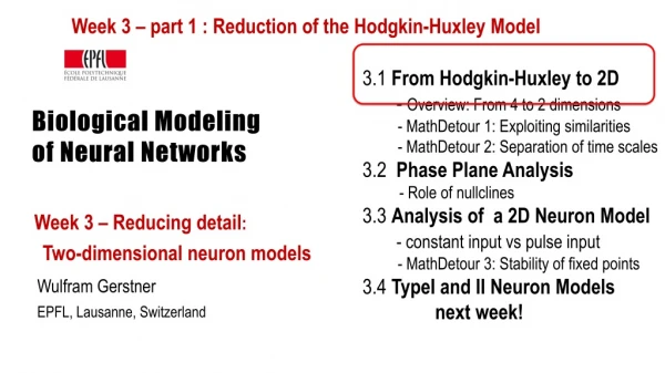
Week 3 – part 1 : Reduction of the Hodgkin-Huxley Model. 3 .1 From Hodgkin-Huxley to 2D - Overview : From 4 to 2 dimensions - MathDetour 1: Exploiting similarities - MathDetour 2: Separation of time scales 3 .2 Phase Plane Analysis

E N D
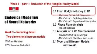
Week 3 – part 1 : Reduction of the Hodgkin-Huxley Model 3.1 From Hodgkin-Huxley to 2D - Overview: From 4 to 2 dimensions - MathDetour 1: Exploitingsimilarities • - MathDetour 2: Separation of time scales 3.2 Phase Plane Analysis • - Role of nullclines 3.3 Analysis of a 2D NeuronModel - constant input vs pulse input • - MathDetour 3: Stability of fixed points 3.4 TypeI and IINeuronModels nextweek! Biological Modelingof Neural Networks Week 3 – Reducing detail: Two-dimensional neuron models Wulfram Gerstner EPFL, Lausanne, Switzerland
Neuronal Dynamics – 3.1. Review :Hodgkin-Huxley Model cortical neuron • Hodgkin-Huxley model • Compartmental models Na+
Neuronal Dynamics – 3.1 Review :Hodgkin-Huxley Model action potential Week 2: Cell membrane contains - ion channels - ion pumps Dendrites (week 4): Active processes? assumption: passive dendrite point neuron spike generation -70mV Na+ K+ Ca2+ Ions/proteins
100 mV 0 • Neuronal Dynamics – 3.1. Review :Hodgkin-Huxley Model inside Ka K Na outside Ion channels Ion pump Reversal potential ion pumpsconcentration difference voltage difference
100 I mV C gK gl gNa 0 stimulus n0(u) u u Neuronal Dynamics – 3.1. Review: Hodgkin-Huxley Model Hodgkin and Huxley, 1952 inside Ka Na outside Ion channels Ion pump 4 equations = 4D system
Neuronal Dynamics – 3.1. Overview and aims Can we understand the dynamics of the HH model? - mathematical principle of Action Potential generation? - constant input current vs pulse input? - Types of neuron model (type I and II)? (next week) - threshold behavior? (next week) Reduce from 4 to 2 equations Type I and type II models ramp input/ constant input f-I curve f-I curve f f I0 I0 I0
Neuronal Dynamics – 3.1. Overview and aims Can we understand the dynamics of the HH model? Reduce from 4 to 2 equations
Neuronal Dynamics – Quiz 3.1. A -A biophysical point neuron model with 3 ion channels, each with activation and inactivation, has a total number of equations equal to [ ] 3 or [ ] 4 or [ ] 6 or [ ] 7 or [ ] 8 or more
Neuronal Dynamics – 3.1. Overview and aims Toward a two-dimensional neuron model • Reduction of Hodgkin-Huxley to 2 dimension • -step 1: separation of time scales • -step 2: exploit similarities/correlations
stimulus m0(u) h0(u) u u Neuronal Dynamics – 3.1. Reduction of Hodgkin-Huxley model MathDetour 1) dynamics of m are fast
Neuronal Dynamics – MathDetour 3.1: Separation of time scales Two coupled differential equations Exercise 1 (week 3) (later !) Separation of time scales Reduced 1-dimensional system Na+
stimulus n0(u) h0(u) u u Neuronal Dynamics – 3.1. Reduction of Hodgkin-Huxley model 1) dynamics of m are fast 2) dynamics of h and nare similar
Neuronal Dynamics – 3.1. Reduction of Hodgkin-Huxley model Reductionof Hodgkin-Huxley Model to 2 Dimension -step 1: separation of time scales -step 2: exploit similarities/correlations Now !
stimulus Neuronal Dynamics – 3.1. Reduction of Hodgkin-Huxley model 2) dynamics of h and nare similar MathDetour u t 1 h(t) hrest nrest n(t) 0 t
Neuronal Dynamics – Detour3.1. Exploit similarities/correlations dynamics of h and nare similar h 1-h Math. argument n 1 h(t) hrest nrest n(t) 0 t
Neuronal Dynamics – Detour3.1. Exploit similarities/correlations dynamics of h and nare similar at rest n 1 h(t) hrest nrest n(t) 0 t
Neuronal Dynamics – Detour3.1. Exploit similarities/correlations dynamics of h and nare similar Rotate coordinate system Suppress one coordinate Express dynamics in new variable n 1 h(t) hrest nrest n(t) 0 t
Neuronal Dynamics – 3.1. Reduction of Hodgkin-Huxley model 2) dynamics of h and nare similar w(t) w(t) 1) dynamics of mare fast
NOW Exercise 1.1-1.4: separation of time scales A: - calculate x(t)! - what if t is small? 0 1 t Exercises: 1.1-1.4 now! 1.5 homework ? t B: -calculate m(t) if t is small! - reduce to 1 eq. Exerc. 9h50-10h00 Next lecture: 10h15
Week 3 – part 1 : Reduction of the Hodgkin-Huxley Model 3.1 From Hodgkin-Huxley to 2D - Overview: From 4 to 2 dimensions - MathDetour 1: Exploitingsimilarities • - MathDetour 2: Separation of time scales 3.2 Phase Plane Analysis • - Role of nullclines 3.3 Analysis of a 2D NeuronModel - constant input vs pulse input • - MathDetour 3: Stability of fixed points 3.4 TypeI and IINeuronModels nextweek! Biological Modelingof Neural Networks Week 3 – Reducing detail: Two-dimensional neuron models Wulfram Gerstner EPFL, Lausanne, Switzerland
Neuronal Dynamics – MathDetour 3.1: Separation of time scales Two coupled differential equations Ex. 1-A Exercise 1 (week 3) Separation of time scales Reduced 1-dimensional system Na+
Neuronal Dynamics – MathDetour 3.2: Separation of time scales Linear differential equation step
Neuronal Dynamics – MathDetour 3.2 Separation of time scales Two coupled differential equations x c I ‘slow drive’ Na+
stimulus n0(u) h0(u) u u Neuronal Dynamics – Reduction of Hodgkin-Huxley model dynamics of m is fast Fast compared to what?
Neuronal Dynamics – MathDetour 3.2: Separation of time scales Two coupled differential equations Exercise 1 (week 3) even more general Separation of time scales Reduced 1-dimensional system Na+
Neuronal Dynamics – Quiz 3.2. A- Separation of time scales: We start with two equations [ ] If then the system can be reduded to [ ] If then the system can be reduded to [ ] None of the above is correct. Attention I(t) can move rapidly, therefore choice [1] not correct
Neuronal Dynamics – Quiz 3.2-similar dynamics Exploiting similarities: A sufficient condition to replace two gating variables r,s by a single gating variable w is [ ] Both r and s have the same time constant (as a function of u) [ ] Both r and s have the same activation function [ ] Both r and s have the same time constant (as a function of u) AND the same activation function [ ] Both r and s have the same time constant (as a function of u) AND activation functions that are identical after some additive rescaling [ ] Both r and s have the same time constant (as a function of u) AND activation functions that are identical after some multiplicative rescaling
Neuronal Dynamics – 3.1. Reduction to 2 dimensions 2-dimensional equation Enables graphical analysis! Phase plane analysis -Discussion of threshold - Constant input current vs pulse input -Type I and II - Repetitive firing
Week 3 – part 1 : Reduction of the Hodgkin-Huxley Model 3.1 From Hodgkin-Huxley to 2D - Overview: From 4 to 2 dimensions - MathDetour 1: Exploitingsimilarities • - MathDetour 2: Separation of time scales 3.2 Phase Plane Analysis • - Role of nullclines 3.3 Analysis of a 2D NeuronModel - constant input vs pulse input • - MathDetour 3: Stability of fixed points 3.4 TypeI and IINeuronModels nextweek! Biological Modelingof Neural Networks Week 3 – Reducing detail: Two-dimensional neuron models Wulfram Gerstner EPFL, Lausanne, Switzerland
stimulus Neuronal Dynamics – 3.2. Reduced Hodgkin-Huxley model
stimulus Neuronal Dynamics – 3.2. Phase Plane Analysis/nullclines 2-dimensional equation Enables graphical analysis! u-nullcline -Discussion of threshold -Type I and II w-nullcline
Neuronal Dynamics – 3.2. FitzHugh-Nagumo Model MathAnalysis, blackboard u-nullcline w-nullcline
Neuronal Dynamics – 3.2. flow arrows Stimulus I=0 Stable fixed point w Consider change in small time step u Flow on nullcline I(t)=0 Flow in regions between nullclines
Neuronal Dynamics – Quiz 3.3 A. u-Nullclines [ ] On the u-nullcline, arrows are always vertical [ ] On the u-nullcline, arrows point always vertically upward [ ] On the u-nullcline, arrows are always horizontal [ ] On the u-nullcline, arrows point always to the left [ ] On the u-nullcline, arrows point always to the right B. w-Nullclines [ ] On the w-nullcline, arrows are always vertical [ ] On the w-nullcline, arrows point always vertically upward [ ] On the w-nullcline, arrows are always horizontal [ ] On the w-nullcline, arrows point always to the left [ ] On the w-nullcline, arrows point always to the right [ ] On the w-nullcline, arrows can point in an arbitrary direction Take 1 minute, continue at 10:55
Neuronal Dynamics – 3.2. Nullclines of reduced HH model stimulus Stable fixed point u-nullcline w-nullcline
stimulus Neuronal Dynamics – 3.2. Phase Plane Analysis 2-dimensional equation Application to neuron models Enables graphical analysis! Important role of - nullclines - flow arrows
Week 3 – part 3: Analysis of a 2D neuron model 3.1 From Hodgkin-Huxley to 2D 3.2 Phase Plane Analysis • - Role of nullcline 3.3 Analysis of a 2D NeuronModel • - pulse input • - constant input • -MathDetour 3: Stability of fixed points 3.4 Type I and II NeuronModels (nextweek)
stimulus Neuronal Dynamics – 3.3. Analysis of a 2D neuron model 2-dimensional equation 2 important input scenarios - Pulse input - Constant input Enables graphical analysis!
Neuronal Dynamics – 3.3. 2D neuron model : Pulse input pulse input
Neuronal Dynamics – 3.3. FitzHugh-Nagumo Model : Pulse input w I(t)=0 u I(t) Pulse input: jump of voltage pulse input
Neuronal Dynamics – 3.3. FitzHugh-Nagumo Model : Pulse input FN model with Image: Neuronal Dynamics, Gerstner et al., Cambridge Univ. Press (2014) Pulse input: jump of voltage/initial condition
Neuronal Dynamics – 3.3. FitzHugh-Nagumo Model DONE! Pulse input: - jump of voltage - ‘new initial condition’ - spike generation for large input pulses w I(t)=0 2 important input scenarios constant input: - graphics? - spikes? - repetitive firing? u Now
Neuronal Dynamics – 3.3. FitzHugh-Nagumo Model: Constant input w-nullcline w I(t)=I0 u • Intersection point (fixed point) • moves • changes Stability u-nullcline
NOW Exercise 2.1: Stability of Fixed Point in 2D w - calculate stability - compare Exercises: 2.1now! 2.2 homework I(t)=I0 u Next lecture: 11:42
Week 3 – part 3: Analysis of a 2D neuron model 3.1 From Hodgkin-Huxley to 2D 3.2 Phase Plane Analysis • - Role of nullcline 3.3 Analysis of a 2D NeuronModel • - pulse input • - constant input • -MathDetour 3: Stability of fixed points 3.4 Type I and II NeuronModels (nextweek)
Neuronal Dynamics – Detour 3.3 : Stability of fixed points. w w-nullcline stable? I(t)=I0 u u-nullcline
stimulus Neuronal Dynamics – 3.3 Detour. Stability of fixed points 2-dimensional equation How to determine stability of fixed point?
stimulus Neuronal Dynamics – 3.3 Detour. Stability of fixed points w I(t)=I0 u unstable saddle stable