Download

1 / 27
270 likes | 396 Vues
Chapter Four Supply and Demand, Applications and Extensions. Linkage Between Resource and Product Markets. Linkage Between Resource and Product Markets. The markets for resources and products are closely linked .

E N D
Linkage Between Resource and Product Markets • The markets for resources and products are closely linked. • In the resource market, businesses demand resources, while households supply them. • Firms demand resources in order to produce goods and services. • Households supply them to earn income. • The labor market is an important resource market.
Linkage Between Resource and Product Markets • An increase in the demand for a product will lead to an increase in the demand for the resources used to produce it. • In contrast, a reduction in the demand for a product will lead to a reduction in the demand for the resources to used produce it. • An increase in the price of a resource will increase the cost of producing products that use it, shifting their supply curve to the left. • A reduction in resource prices will have the opposite affect.
S2 S2 S1 Price(wage) ResourcesMarket Resource Prices and Product Markets S1 • Suppose there is a reduction in the supply of young workers … • The higher wages increase the restaurant’s cost, causing a reduction in supply in the product market … $10 $8 which pushes the wages of restaurant waiters / waitress up. DR Employment(wait staff) E2 E1 leading to higher meal prices. ProductMarket Price $12 $11 DP Quantity(of meals) Q1 Q2
Price Ceilings • A price ceiling establishes a maximum price that sellers are legally permitted to charge. • Example: rent control • When a price ceiling keeps the price of a good below market equilibrium, there will be both direct and indirect effects. • (Direct effect) Shortage: the quantity demanded will exceed the quantity supplied. Waiting lines may develop. • (Indirect effects) Quality deterioration and changes in other non-price factors favorable to sellers & unfavorable to buyers. • The quantity exchanged will fall and the gains from trade will be less than if the good were allocated by markets.
Price ceiling Shortage Impact of a Price Control • Consider the rental housingmarketwhere the price (rent) P0would bring the quantity of rental units demandedinto balance with the quantity supplied. Rental housing market Price(rent) S • A price ceilinglike P1 imposes a price below market equilibrium … P0 causing quantity demanded QD… to exceed quantity supplied QS … resulting in a shortage. P1 • Because prices are not allowed to direct the market to equilibrium, non-price elements will become more important in determining where the scarce goods go. D Quantity of housing units QS QD
Effects of Rent Control • Shortages and black markets will develop. • The future supply of housing will decline. • The quality of housing will deteriorate. • Non-price methods of rationing will increase in importance. • Inefficient use of housing will result. • Long-term renters will benefit at the expense of newcomers.
Price Floor • A price floor establishes a minimum legal price for the good or service. • Example: minimum wage • When a price floor keeps the price of a good above the market equilibrium, it will lead to both direct and indirect effects. • (Direct effect) Surplus: sellers will want to supply a larger quantity than buyers are willing to purchase. • (Indirect effects) Changes in non-price factors favorable to buyers and unfavorable to sellers. • The quantity exchanged will fall and the gains from trade will be less than if the good were allocated by markets.
Surplus Price floor Impact of a Price Floor Price S • A price floorlike P1 imposes a price above market equilibrium … P1 causing quantity supplied Qs … to exceed quantity demanded QD … resulting in a surplus. P0 • Because prices are not allowed to direct the market to equilibrium, non-price elements of exchange will become more important in determining where scarce goods go. D Quantity QD QS
Minimum Wage: An Example of a Price Floor • When the minimum wage is set above the market equilibrium for low-skill labor, the following will occur: • Direct effect: • Reduces employment of low-skilled labor. • Indirect effects: • Reduction in the non-wage components of compensation • Less on-the-job training • May encourage students to drop out of school
Excess Supply Minimum wage level Employment and the Minimum Wage Low-skilllabor market Price(wage) • Consider the market for low-skilllaborwhere a price (wage) of $5 could bring the quantity of labor demandedinto balance with the quantity supplied. S $7.25 $5.00 • A minimum wage(price floor) of $7.25 would increase the wages of low-skill labor, but employment will decline from E0 to E1. • Those who lose their jobs will be pushed into either unemployment or less preferred employment. D Quantity(low-skill employment) E1 E0
Does the Minimum Wage Help the Poor? • While increasing the minimum wage will increase the wages of low-skill workers, their on-the-job training opportunities, non-wage benefits, working conditions, and employment will decline. • Who earns minimum wage? • Most minimum wage workers are young and / or only working part-time. • Fewer than 20 percent are from families with incomes below the poverty line.
Black Markets • Black market:A market that operates outside the legal system. • The primary sources of black markets are: • Evasion of a price control • Evasion of a tax (e.g. high excise taxes on cigarettes) • Legal prohibition on the production and exchange of a good (e. g., prostitution, marijuana and cocaine) • Black markets have a higher incidence of defective products, higher profit rates, and greater use of violence to resolve disputes.
Importance of the Legal System • A legal system that provides secure property rights and an unbiased enforcement of contracts enhances the operation of markets. • Markets will exist in any environment, but they can be counted on to function efficiently only when property rights are secure and contracts enforced in an evenhanded manner. • The inefficient operation of markets in countries like Russia following the collapse of communism illustrates the importance of an even-handed legal system.
Average Tax Rate • The average tax rate equals tax liability divided by taxable income. • A progressive tax is one in which the average tax rate rises with income. • A proportional tax is one in which the average tax rate stays the same across income levels. • A regressive tax is one in which the average tax rate falls with income.
Marginal Tax Rate • The marginal tax rateis calculated as the change in tax liability divided by the change in taxable income. • The marginal tax rate is highly important because it determines how much of an additional dollar earned must be paid in taxes (and therefore, how much one gets to keep). In this way, the marginal tax rate directly impacts an individual’s incentive to earn.
35000 35050 4938 4938 4416 4656 35050 35100 4950 4950 4424 4664 35100 35150 4963 4963 4431 4671 35150 35200 4975 4975 4439 4679 35200 35250 4988 4988 4446 4686 35250 35300 5000 5000 4454 4694 35300 35350 5013 5013 4461 4701 35350 35400 5025 5025 4469 4709 35400 35450 5038 5038 4476 4716 35450 35500 5050 5050 4484 4724 35500 35550 5063 5063 4491 4731 35550 35600 5075 5075 4499 4739 Marginal Tax Rate 2010 Tax Table Continued If line 43(taxableincome) is And you are • An excerpt from the 2010 federal income tax table is shown here. Single Married filing jointly Married filing separately Head of a house- hold • Note, for single individuals, as income increases from $35,000 to $35,100 … But less than Atleast Your tax is … their tax liability increases from $4,938 to $4,963. $33,000 • In this range, what is the individual’s marginal tax rate? • What is the individual’s average income tax rate?
Tax Rate and Tax Base • Tax rate:defined as the rate (%) at which an activity is taxed. • Tax base: defined as the amount of the activity that is taxed. • Note: the tax base is inversely related to the rate at which the activity is taxed. • Tax revenues:defined as tax rate multiplied by tax base.
Laffer Curve • The Laffer curve(next page) illustrates the relationship between tax rates and tax revenues. • As tax rates increase from low levels, tax revenues will also increase even though the tax base is shrinking. • As rates continue to increase, at some point, the shrinkage in the tax base will dominate and the higher rates will lead to a reduction in tax revenues. • The Laffer Curve shows that tax revenues are low for both high and low tax rates.
C B A The Laffer Curve • At a tax rate of 0%, tax revenues would also be equal to $0. Tax rate(percent) • At a tax rate of 100%, nobody would work, and so, tax revenues would be equal to $0. 100 • As the tax rate increases from 0% to some level like A, tax revenues increase despite the fact some individuals work less. 75 • As rates continue to increase (beyond B, for example), higher rates will eventually cause revenues to fall. 50 • Still higher tax rates will lead to even less tax revenue (from Bto C and beyond). This is because the tax base shrinks faster than the increased revenues from higher tax rates. 25 • There is no presumption that the level of the tax rate at Bis the ideal tax rate, only that Bmaximizes tax revenue in the current period. Tax revenues 0 Maximum
Laffer Curve & Tax Changes in the 1980s • During the 1980s, the top Federal marginal income tax rate fell from 70% to 33%. • It is important to distinguish between changes in tax rates and changes in tax revenues. • Even though the top Federal income tax rates were cut sharply during the 1980s, the tax revenues and the share of personal income tax paid by high earners rose during the decade. See the following slide for details.
192 153 153 149 87 1980 58 1990 Changes in Taxes Paid in the 1980s • Measured in 1982-1984 dollars, personal income taxes paid by the top 1 and 10 percent of income recipients increased between 1980 and 1990 even though their rates were reduced. • Tax revenues collected from the other taxpayers were virtually unchanged during the decade. Personal Income Taxes Paid(by income group, billions of 1982-1984 $) Top 1% Other 90% Top 10%
End of Chapter 4