Download
1 / 28
280 likes | 300 Vues
This study presents findings from 3D simulations of 85 earthquakes on 10 faults, with variations in rupture scenarios. The analysis includes basin response parameterization and comparison with 1D simulations. The study evaluates basin depth effects, synthetic time histories, and basin-edge impacts. Results suggest period-dependent variability in mean and variance, with the reduction of under-prediction at long periods. Potential for basin-specific and event-specific variations is noted for future research.

E N D
Parameterization of Basin Response Based on 3D Simulations by PEER/SCEC 3D Ground Motion Project Team PI: Steven M. Day San Diego State University March 25, 2004
Simulations Completed • 85 different earthquake simulations • 10 faults from SCEC Community Fault Model • 6 rupture scenarios for each (hypocenter and slip model variations) • 10 cross-check simulations (1 per fault) • 15 1D reference simulations
Faults Modeled • 1. Sierra Madre (7.0) • 2. Santa Monica SW (6.3) • 3. Hollywood (6.4) • 4. Raymond (6.6) • 5. Puente Hills I (6.8) • 6. Puente Hills II (6.7) • 7. Puente Hills (all) (7.1) • 8. Compton (6.9) • 9. Newport-Inglewood (6.9) • 10. Whittier (6.7)
Six Rupture Scenarios Per Fault • 2 hypocenters • 1/4 fault-length from each end • 7/10 fault-width down dip • 3 slip models • Constructed following Somerville (1999) • Constant rupture velocity (2.8 km/s) • Rise time scaled to empirical formula: Log(Tr)=0.5(Mw+10.7) + log(2.9x10⁻⁹)
Coordination Scheme R = 1D rock reference simulation S = 1D basin-profile simulation F = 6 3D scenarios C = single cross-check
Output • Full time histories • 3 velocity components • 1600 surface points per simulation • Basin and rock sites sampled • ~300,000 synthetic time histories and associated metadata in digital library
Cross-check (cont’d) • Sierra Madre Scenario • Compares FD and FE codes at 16 sites (N-S component): • FD (UCB/LLNL) red • FE (CMU) green
Response Spectra Data Set • synthetic Sa ordinates (2-10 second period range) • source distances • local basin depth measures (depths to 1.0, 1.5, 2.5, and 3.5 km/s isosurfaces) • Sa files available on web
3D÷1D_rock Sa Ratios ln(Sa Ratio) Frequency (Hz) Frequency (Hz)
Vertically Incident SH Response ln(Sa Ratio) Frequency (Hz) Frequency (Hz)
Curve Fits to Basin Depth Effect(Separately Optimized at Each Period)
Curve Fits to Basin Depth Effect(6-parameter model for Depth and Period Dependence)
Basin Effect Relative to 1-D Soil (2000 m Depth to Isosurface)
1D Rock Simulations vs A-S Regression Model Underprediction Factor Period (sec)
Transfer Function from “Very Hard Rock” to Boore/Joyner “Generic Rock”
Summary • Source-averaged 3D effect is largely captured by basin depth term (depth to 1.5 km/s isosurface) • Mean and variance are period-dependent • Results almost certainly double-count effects partially represented in “rock” regression equations • With ~500 m depth sites (instead of 0 depth) taken as “rock” reference: • absolute amplitudes at long period (5 sec) come into agreement with A-S rock regression (i.e., under-prediction eliminated) • Addition under-prediction at shorter periods probably partly a source effect (which would be removed by our analysis of ratios) • Maximum basin effect reduced to ~2 (@ 2 sec) to ~3 (@ 10 sec)
Summary (cont’d) • Little or no systematic basin-edge effect in source-averaged residuals • Likewise, no clear basin-edge effect in source-averaged standard deviations
Directions for Additional Work • Analysis of current synthetic data set for • Basin-specific (e.g., L.A., San Fernando, San Gabriel) variations • Event-specific basin effects • Simulations for additional regions (e.g., Santa Clara Valley? Imperial Valley? others) to examine transportability of results • Push simulations to ~1 Hz