Download
1 / 66
680 likes | 779 Vues
Learn about estimation techniques and inference methods in the marginal model, including ML and REML estimation, mean and variance components inference, and fitting linear mixed models in SAS. Explore the 2-stage model formulation and the general linear mixed-effects model. Dive into examples and estimation processes, including ML and REML estimates, contrast variables, and inference for the mean structure using Approximate Wald tests and likelihood ratio tests.

E N D
Lecture 2Estimation and Inference for the marginal model Ziad Taib Biostatistics, AZ April 2011 Name, department
Outline of lecture 2 • A reminder • Estimation for the marginal model ML and REML estimation • Inference for the mean structure • Inference for the variance components • Fitting linear mixed models in SAS Name, department
1. A reminder: The 2-stage Model Formulation: Name, department
Stage 1 • Response Yij for ith subject, measured at time tij,i = 1, . . . , N, j = 1, . . . , ni • • Response vector Yifor ith subject: • Ziis a (nix q) matrix of known covariates and • biis a (nix q) matrix of parameters • Note that the above model describes the observed variability within subjects Possibly after some convenient transformation Name, department
Stage 2 • Between-subject variability can now be studied from relating the parameters bito known covariates • Kiis a (qx p) matrix of known covariates and • bis a (p-dimensional vector of unknown regression parameters • Finally Name, department
The General Linear Mixed-effectsModel • The 2-stages of the 2-stage approach can now be combined into one model: Average evolution Subject specific Name, department
The hierarchical versus the marginal Model It can be written as The general mixed model is given by It is therefore also called a hierarchical model Name, department
Marginally we have that is distributed as Hence f(yiI bi) f(bi) f(yi) Name, department
Example Name, department
The prostate data A model for the prostate cancer Stage 1 Name, department
The prostate data A model for the prostate cancer Stage 2 Age could not be matched Ci, Bi, Li, Miare indicators of the classes: control, BPH, local or metastatic cancer. Agei is the subject’s age at diagnosis. The parameters in the first row are the average intercepts for the different classes. Name, department
The prostate data This gives the followingmodel eij Name, department
2. Estimation in the Marginal Model: ML and REML Estimation Name, department
ML and REML estimates: Name, department
ML and REML estimates (cont’d) Name, department
Estimation based on the marginal model Vi Name, department
ML estimation • Maximise with respect to b • Replace in the likelihood function • Maximise with respect to a • One can use the EM algorithm or Newton Raphson Name, department
ML estimation Name, department
REML ESTIMATION • Restricted (or residual, or reduced) maximum likelihood (REML) approach is a particular form of maximum likelihood estimation which does not base estimates on a maximum likelihood fit of all the information, but instead uses a likelihood function calculated from a transformed set of data, so that nuisance parameters have no effect. • In the case of variance component estimation, the likelihood function is calculated from the probability distribution of a set of contrasts. In particular, REML is used as a method for fitting linear mixed models. In contrast to maximum likelihood estimation, REML can produce unbiased estimates of variance and covariance parameters. Name, department
Analysis of Contrast Variables Contrast variables in repeated measures data are linear combinations of the responses over time for an individual. In longitudinal studies it is of interest to consider the set of differences between responses at consecutive time points, that is, changes from time 1 to time 2, time 2 to time 3, and so forth. A set of contrast variables can be used to analyze trends over time and to make comparisons between times. The original repeated measures data for each individual are transformed into new sets of variables each given by a set of contrast variables. Name, department
REML estimation • Given an iid sample Yii = 1, . . . , N, we can estimate the variance using • But since m is uknown, we use • Based on this we can define Name, department
REML Name, department
3. Inference for the meanstructure Name, department
Approximate Wald tests • Under the Wald statistical test, named after Abraham Wald, the maximum likelihood estimate of the parameter(s) of interest b is compared with the proposed value b0, with the assumption that the difference between the two will be approximately normal. Typically the square of the difference is compared to a chi-squared distribution. In the univariate case, the Wald statistic is • which is compared against a chi-square distribution. Alternatively, the difference can be compared to a normal distribution. In this case the test statistic is Name, department
Approximate Wald tests Obs!a is estimated which gives extra variability and bias. Bias is resolved by using t- or F-test. Name, department
Approximate t-and F- tests Name, department
Robust inference Name, department
Likelihood ratio tests Name, department
Likelihood ratio tests Name, department
4. Inference for the Variance Components Name, department
5. Fitting linear mixed models in SAS Name, department
Statistical software Name, department
Software (cont’d) • SAS – SPSS – BMDP/5v – ML3 – HLM – Splus – R can handle correlated data but some are more restricted than others. • Most packages offer a choice between ML and REML and optimisation is often based on Newton-Raphson, the EM algorithm or Fisher scoring. • The user has to specify a model for the mean response that is linear in the fixed effects and to specify a covariance structure. The user can select a full parameterisation of the covariance structure (unstructured) or choose among given covariance structures. • The covariance structure is also influenced by the inclusion of random effects and their covariance structure. Name, department
Software (cont’d) • Output often includes: • history of optimisation iterations • estimates of fixed effects • covariance parameters with standard errors • estimates of user specified contrasts • Graphics is often limited but can be done in another software Name, department
SAS PROC MIXED and Repeated Measures • PROC MIXED of SAS offers greater flexibility for the modelling of repeated measures data than PROC GLM. (Firstly, the procedure provides a mechanism for modelling the covariance structure associated with the repeated measures. Secondly, it can handle some forms of missing data without discarding an entire subject’s-worth of data. Thirdly, it has some capability to handle the situation when each subject may be measured at different times and time intervals.) • In PROC GLM, repeated measures are handled in a multivariate framework and it requires a multivariate view of the data. PROC MIXED, on the other hand, requires a univariate or stacked-data view of the data. In other words, there is only a single response variable. The repeated information, including all of the information about the subjects, is contained in other variables. Proc GLMassumes that the covariance matrix meets a sphericity assumption compound symmetry. Name, department
SAS PROC MIXED • Proc mixed was designed to handle mixed models. It has a large choice of covariance structures (unstructured, random effects, autoregressive, Diggle etc) • PROC MIXED can be used not only to estimate the fixed parameters, but also the covariance parameters. • By default, PROC MIXED estimates the covariance parameters using the method of restricted maximum likelihood (REML). • PROC MIXED provides empirical Bayes estimates. • Separate analyses for separate groups can be run using the BY statement. • Approximate F tests for class variables are obtained using Wald’s test. • All components of the output can be saved as a SAS data set for further manipulation using other internal (SAS) or external procedures. Name, department
PROC MIXED: Syntax PROC MIXED < options > ; BY variables ; CLASS variables ; ID variables ; MODEL dependent = < fixed-effects > < / options > ; RANDOM random-effects < / options > ; REPEATED < repeated-effect > < / options > ; PARMS (value-list) ... < / options > ; PRIOR < distribution > < / options > ; CONTRAST 'label' < fixed-effect values ... > < | random-effect values ... > , ... < / options > ; ESTIMATE 'label' < fixed-effect values ... > < | random-effect values ... >< / options > ; LSMEANS fixed-effects < / options > ; MAKE 'table' OUT=SAS-data-set ; WEIGHT variable ; Name, department
In Proc Mixed, the mixed model is specified by means of a number of statements like CLASS, MODEL, RANDOM and REPEATED. • The CLASS statement identifies the classification variables (for example, gender, person, age, etc.). • The MODEL statement specifies the model’s fixed effects equation, Xiβ. Thus, the design matrix Xi is defined and the model’s intercept is included by default. • The RANDOM statement isused to specify random effects and the form of covariance matrix D. (Useful options: SOLUTION: print random effects solution). • The REPEATED statement models the intra-individual variation and includes the structure of Si=Cov(ei), where Siis a block diagonal matrix for each subject. (If the REPEATED statement is not included it is assumed that Si=σ2I). • LSMEANS Calculates least squares mean estimates of specified fixed effects. Name, department
Modelling the Covariance Structure Using the RANDOM and REPEATED Statements in PROC MIXED Measures on different individuals are independent, so covariance needs attention only with measures on the same individuals. The covariance structure refers to variances at individual times and to correlation between measures at different times on the same individual. There are basically two aspects of the correlation. • First, two measures on the same individual are correlated simply because they share common contributions from that individual. This is due to variation between indivduals. • Second, measures on the same individual close in time are often more highly correlated than measures far apart in time. This is covariation within indivduals. . Usually, when using PROC MIXED, the variation between indivduals is specified by the RANDOM statement, and covariation within indivduals is specified by the REPEATED statement Name, department
PROC MIXED fits many different structures (some are listed here). Note also that a particular structure may be fit using more than one “TYPE” designation, and with combinations of the RANDOM and REPEATED statements. Name, department
Data structure of Proc Mixed • Consider the example where arm strength is measured on 8 patients at 3 different times and where patients have been randomized to one of 2 treatment groups. The multivariate view associated with e.g. PROC GLM code: would look like below Name, department