Download
1 / 46
460 likes | 627 Vues
Scientific Carbon Stochastic Volatility Model Estimation and Inference: Forecasting (Un-)Conditional Moments for Options Applications by Per Bjarte Solibakke a a) Department of Economics, Molde University College. Background and Outline

E N D
Scientific Carbon Stochastic Volatility Model Estimation and Inference: Forecasting (Un-)Conditional Moments for Options Applications by Per BjarteSolibakkea a) Department of Economics, Molde University College CFE-2011, Parallel Sessions, Monday 19/12/2011
Background and Outline • The Front December Future Contracts NASDAQ OMX: phase II 2008-2012 • No existence of EUAs spot-forward relationship does not exist • EUA options have carbon December futures as underlying instrument • Price dynamics are depending on total emissions • 2. The dynamics of the forward rates are directly specified. • The HJM-approach adopted to modelling forward- and futures prices in commodity markets. • Alternatively, we model only those contracts that are traded, resembling swap and LIBOR models in the interest rate market ( also known as market models). Construct the dynamics of traded contracts matching the observed volatility term structure. • The EUA options market on carbon contract are rather thin, we will therefore estimate the option prices on the future prices themselves. Black-76 / MCMC simulations. CFE-2011, Parallel Sessions, Monday 19/12/2011 Page: 2
Background and Outline (cont.) • 3. Stochastic Model Specification, Estimation, Assessment and Inference • 4. Forecasting unconditional Futures and Options Moments, • and measures for risk management and asset allocation • 5. Forecasting conditional Futures and Options Moments • i. One-step-ahead Conditional Mean (expectations) • ii. One-step-ahead Standard deviation / Particle filtering • iii. Multi-step-ahead Mean and Volatility Dynamics • iv. Mean / Volatility Persistence • 6. Conditional Risk Management and Asset Allocation Measures • 7. The EMH case for CARBON commodity markets CFE-2011, Parallel Sessions, Monday 19/12/2011 Page: 3
The Carbon NASDAQ OMX commodity market NASDAQ OMX commodities provide access to one of Europe’s leading carbon markets. 350 members from 18 countries covering a wide range of energy producers, consumers and financial institutions. Members can trade cash-settlement derivatives contracts in the Nordic, German, Dutch and UK power markets with futures, forward, option and CfD contracts up to six years’ duration including contracts for days, weeks, months, quarters and years. The reference price for the power derivatives is the underlying day-ahead price as published by Nord Pool spot (Nordics), the EEX (Germany), APX ENDEX (the Netherlands), and N2EX (UK). CFE-2011, Parallel Sessions, Monday 19/12/2011 Page: 4
Indirect Estimation and Inference: Projection: The Score generator (A Statistical Model) establish moments: the Mean (AR-model) the Latent Volatility ((G)ARCH-model) Hermite Polynomials for non-normal distribution features Estimation: The Scientific Model – A Stochastic Volatility Model The General Scientific Model methodology (GSM): SDE: where z1t , z2t and (z3t ) are iid Gaussian random variables. The parameter vector is: A vector SDE with two stochastic volatility factors. CFE-2011, Parallel Sessions, Monday 19/12/2011 Page: 5
The General Scientific Model methodology (GSM): • Re-projection and Post-estimation analysis: • MCMC simulation for Option pricing, Risk Management and Asset allocation • Conditional one-step-ahead mean and volatility densities. • Forecasting volatility conditional on the past observed data; and/or • extracting volatility given the full data series (particle filtering) • The conditional volatility function, Multi-step-ahead mean and volatility • and mean/volatility persistence. Other extensions. Applications: Andersen and Lund (1997): Short rate volatility Solibakke, P.B (2001): SV model for Thinly Traded Equity Markets Chernov and Ghysel (2002): Option pricing under Stochastic Volatility Dai & Singleton (2000) and Ahn et al. (2002): Affine and quadratic term structure models Andersen et al. (2002): SV jump diffusions for equity returns Bansal and Zhou (2002): Term structure models with regime-shifts Gallant & Tauchen (2010): Simulated Score Methods and Indirect Inference for Continuous-time Models CFE-2011, Parallel Sessions, Monday 19/12/2011 Page: 6
Stochastic Volatility Models: Simulation-based Inference Early references are: Kim et al. (1998), Jones (2001), Eraker (2001), Elerian et al. (2001), Roberts & Stamer (2001) and Durham (2003). A successful approach for diffusion estimation was developed via a novel extension to the Simulated Method of Moments of Duffie & Singleton (1993). Gouriéroux et al. (1993) and Gallant & Tauchen (1996) propose to fit the moments of a discrete-time auxiliary model via simulations from the underlying continuous-time model of interest. The idea (Bansal et al., 1993, 1995 and Gallant & Lang, 1997; Gallant & Tauchen, 1997): Use the expectation with respect to the structural model of the score function of an auxiliary model as the vector of moment conditions for GMM estimation. Replacing the parameters from the auxiliary model with their quasi-maximum likelihood estimates, leaves a random vector of moment conditions that depends only on the parameters of the structural model. CFE-2011, Parallel Sessions, Monday 19/12/2011 Page: 7
Simulated Score Methods and Indirect Inference for Continuous-time Models (some details): Estimation Simulated Score Estimation: Suppose that: is a reduced form model for observed time series, where xt-1 is the state vector of the observable process at time t-1 and yt is the observable process. Fitted by maximum likelihood we get an estimate of the average of the score of the data satisfies: That is, the first-order condition of the optimization problem. Having a structural model (i.e. SV) we wish to estimate, we express the structural model as the transition density , where q is the parameter vector. It can be relatively easy to simulate the structural model and is the basic setup of simulated method of moments (Duffie and Singleton, 1993; Ingram and Lee, 1991). CFE-2011, Parallel Sessions, Monday 19/12/2011 Page: 8
Simulated Score Methods and Indirect Inference for Continuous-time Models (some details): Structural Model Estimation • The scientific model is built using financial market insight/knowledge • Stochastic volatility model computable from a simulation • Metropolis-Hastings algorithm to compute the posterior (only need of a function proportional to the prior) Details for parameter q estimation: Compute: where denotes the observed data and n is the sample size. Given a current and the corresponding we obtain the pair as follows (the M-H algorithm): Draw according to Simulate according to Compute and (parameter functionals) from simulation Define With probability otherwise Page: 9
Main question: How do the results change as the prior is relaxed? That is: How does the marginal posterior distribution of a parameter or functional of the statistical model change? Distance measurement: where Aj is the scaling matrices. Simulated Score Methods and Indirect Inference for Continuous-time Models (some details): Assessment For a well fitting scientific model: The location measure should not move by a scientifically meaningful amount as k increases. However, the scale measure can increase. Page: 10
Simulated Score Methods and Indirect Inference for Continuous-time Models (some details): Re-projection / Post-Estimation Analysis Elicit the dynamics of the implied conditional density for observables: The unconditional expectations can be generated by a simulation: Let . Theorem 1 of Gallant and Long (1997) states: We study the dynamics of by using as an approximation. CFE-2011, Parallel Sessions, Monday 19/12/2011 Page: 11
Application: Financial CARBON Contracts (EUA) NORD POOL (Phase II: 2008-2012) Front December Futures Contracts (EUA options will have the December futures as the underlying instrument) CFE-2011, Parallel Sessions, Monday 19/12/2011
Objectives (purpose): • Higher Understanding of the Carbon Futures Commodity Markets • the Mean equations • the Volatility equations • Models derived from scientific considerations and theory is always • preferable • Fundamentals of Stochastic Volatility Models • Likelihood is not observable due to latent variables (volatility) • The model is continuous but observed discretely (closing prices) • Bayesian Estimation Approach is credible (densities) • Accepts prior information • No growth conditions on model output or data • Estimates of parameter uncertainty (distributions) is credible • Financial Contracts Characteristics and Risk Assessment & Management • The Financial Contracts Characteristics CFE-2011, Parallel Sessions, Monday 19/12/2011 Page: 13
Objectives (purpose): (cont) • Value-at-Risk / Expected Shortfall for Risk Management • Stochastic Volatility models are well suited simulation • Using Simulation and Extreme Value Theory for VaR-/CVaR-Densities • Simulations and Greek Letters Calculations for Asset Allocation • Direct path wise hedge parameter estimates • MCMC superior to finite difference, which is biased and time-consuming • Re-projection for Simulations and Forecasting (conditional moments) • Conditional Mean and Volatility forecasting • Volatility Filtering • The Case against the Efficiency of FutureMarkets (EMH) • Serial correlation in Mean and Volatility • Price-Trend-Forecasting models and Risk premiums • Predictability CFE-2011, Parallel Sessions, Monday 19/12/2011 Page: 14
Objectives (why): SV models has a simple structure and explain the major stylized facts. Moreover, market volatilities change so frequent that it is appropriate to model the volatility process by a random variable. Note, that all model estimates are imperfect and we therefore has to interpret volatility as a latent variable (not traded) that can be modelled and predicted through its direct influence on the magnitude of returns. Mainly three motivational factors: 1. Unpredictable event on day t; proportional to the number of events per day. (Taylor, 86) 2. Time deformation, trading clock runs at a different rate on different days; the clock often represented by transaction/trading volume (Clark, 73). 3. Approximation to diffusion process for a continuous time volatility variable; (Hull & White (1987) CFE-2011, Parallel Sessions, Monday 19/12/2011 Page: 15
Objectives (why): Other motivational factors: 4. A model of futures markets directly, without considering spot prices, using HJM-type models. A general summary of the modelling approaches for forward curves can be found in Eydeland and Wolyniec (2003). Matching the volatility term structure. 5. In order to obtain an option pricing formula the futures are modelled directly. Mean and volatility functions deriving prices of futures as portfolios. Such models can price standardized options in the market. Moreover, the models can provide consistent prices for non-standard options. 6. Enhance market risk management, improve dynamic asset/portfolio pricing, improve market insights and credibility, making a variety of market forecasts available, and improve scientific model building for commodity markets. CFE-2011, Parallel Sessions, Monday 19/12/2011 Page: 16
Carbon Application MCMC estimation/inference: • 1. NASDAQ OMX Carbon front December contracts • 2. The Statistical model and the Stochastic Volatility Model • 3. Model assessment (relaxing the prior): model appropriate? • Empirical Findings in the mean and latent volatility. • Unconditional mean and latent volatility paths/distributions • Carbon Post-Estimation Analysis: • 1. SV-model simulations: Option prices, Risk management and Asset Allocation (unconditional). • 2. Conditional mean and volatility, particle filtering, variance functions, • multi-step ahead dynamics and persistence. • Conditional Risk Management and Asset Allocation • EMH and Model Summary/Conclusion Data Characteristics Estimation Results Assessment Model Findings Risk M/Asset Alloc Re-projection/Post-Est Conditional Moments EMH/ Model Summary CFE-2011, Parallel Sessions, Monday 19/12/2011 Page: 17
Back to Overview CFE-2011, Parallel Sessions, Monday 19/12/2011
Return Application Carbon Front December Contracts Carbon front December Contracts: Page: 19
Back to Overview CFE-2011, Parallel Sessions, Monday 19/12/2011
Return Application Carbon Front December Contracts Scientific Models: Stochastic Volatility Model /Parameters (q) Bayesian Estimation Results 1. Several serial Bayesian runs establishing the mode We tune the scientific model until the posterior quits climbing and it looks like the mode has been reached: 2. A final parallel run with 24 (8 *3) CPUs and 240.000 MCMC simulations (OPEN_MPI (Indiana University) parallell computing) CFE-2011, Parallel Sessions, Monday 19/12/2011 Page: 21
Back to Overview CFE-2011, Parallel Sessions, Monday 19/12/2011
Application Carbon Front December Contracts Scientific Model: Model Assessment – the model concerttest Carbon front December k = 1, 10, 20 and 100 densities – reported. Page: 23
Application Carbon Front December Contracts Scientific Model: The Stochastic Volatility Model: log-sci-mod-posterior Log sci-mod-posterior (every 25th observation reported): Optimum is along this path! Page: 24
Application Carbon Front December Contracts Scientific Model: Carbonq-paths and densities; 240.000 simulations Page: 25
Return Application Carbon Front December Contracts • Scientific Model: Stochastic Volatility The chains look good. Rejection rates are: The MCMC chain has found its mode. • A well fitted scientific SV model: • The result indicates that the model fits and that location measure is stable and the scale measure increases, indicating that the scientific model has empirical content. CFE-2011, Parallel Sessions, Monday 19/12/2011 Page: 26
Back to Overview CFE-2011, Parallel Sessions, Monday 19/12/2011
Return Application Carbon Front December Contracts Empirical Model Findings: • For the mean stochastic equation: • Positive mean drift (a0 = 0.026; s.e. = 0.03) and serial correlation (a1 = 0.054; s.e. 0.021) for the CARBON contracts • For the latent volatility: two stochastic volatility equations: • Positive constant parameter (e0.6305 >> 1) • Two volatility factors (s1 = 0.0624, s.e.=0.0161; s2 = 0.2263, s.e.=0.0329) • Persistence is high for s1 with associated (b1 = 0.985, s.e. = 0.0381) ; persistence is lower for s2 with associated (b2 = 0.5775, s.e.=0.0806) • Asymmetry is strong and negative (r1 = -0.4324, s.e.=0.1130) Page: 28
Back to Overview CFE-2011, Parallel Sessions, Monday 19/12/2011
Application Carbon Front December Contracts Scientific Model: The Stochastic Volatility Model. The Option market versus SV-model prices 05.09.2011 Page: 30
Application Carbon Front December Contracts Scientific Model: The Stochastic Volatility Model. Risk assessment and management: CARBON VaR / CVaR Page: 31
Return Application Carbon Front December Contracts Scientific Model: The Stochastic Volatility Model. Asset Allocation/Dynamic Hedging: CARBON GREEK Letters Page: 32
Back to Overview CFE-2011, Parallel Sessions, Monday 19/12/2011
Application Carbon Front December Contracts Scientific Model: Re-projections / nonlinear Kalman filtering Of immediate interest of eliciting the dynamics of observables: One-step ahead conditional mean: One-step ahead conditional volatility: Filtered volatility is the one-step ahead conditional standard deviation evaluated at data values: where yt denotes the data and yk0 denotes the kth element of the vector y0, k = 1,…M. For instance, one might wish to obtain an estimate of: for the purpose of pricing an option (from the re-projection step). CFE-2011, Parallel Sessions, Monday 19/12/2011 Page: 34
Application Carbon Front December Contracts SV Model: One-step-ahead conditional moments Page: 35
Application Carbon Front December Contracts SV Model: filtered volatility /particle filtering for Option pricing Page: 36
Application Carbon Front December Contracts SV Model: Conditional variance functions (asymmetry) (shocks to a system that comes as a surprise to the economic agents) Page: 37
Application Carbon Front December Contracts SV Model: Multistep-ahead volatilitydynamics (volatility impulse-response profiles) CFE-2011, Parallel Sessions, Monday 19/12/2011 Page: 38
Return Application Carbon Front December Contracts SV Model: Mean and Volatility Persistence (half-lives = –ln2 / b) CFE-2011, Parallel Sessions, Monday 19/12/2011 Page: 39
Back to Overview CFE-2011, Parallel Sessions, Monday 19/12/2011
Application Carbon Front December Contracts • Scientific Model Re-projections: Conditional SV-model moments: Conditional VaR/CVaR for RM and Greeks for Asset allocation CFE-2011, Parallel Sessions, Monday 19/12/2011 Page: 41
Return Application Carbon Front December Contracts • Scientific Model Reprojections: Extensions using SV-model simulations: Realized Volatility and continuous / jump volatility (5 minutes simulations): CFE-2011, Parallel Sessions, Monday 19/12/2011 Page: 42
Return Application Carbon Front December Contracts • Scientific Model Re-projections: Post Estimation Analysis • Post estimation analysis add new information to market participants: • Option prices for any derivative for any maturity. Credible densities are available for all call/put prices. • Credible densities for VaR/CVaR and Greek letters are available for risk management and asset allocation • Conditional mean (expectations) is narrow information from the history? • The filtered volatility (particle filter) add information for the one-day-ahead conditional volatility. Conditional return densities for obs. Xt-1.Gauss quadrature densities are available. • Conditional variance functions evaluates the surprise to economic agents from market shocks. • Multi-step-ahead dynamics for the mean and volatility are available • Conditional Risk management and asset allocation measures available • Realized Volatility can be obtained from simulation step change (96 steps per day = 5 minutes data). Page: 43
Back to Overview CFE-2011, Parallel Sessions, Monday 19/12/2011
Application Carbon Front December Contracts CARBON front December contracts and EMH: • Drift in the mean (risk premium) is positive but negligible (insignificant) • The positive serial correlation in the mean (0.054) is probable not tradable • The volatility clustering is strong (0.985) but probably not tradable • Asymmetry is strong (-0.432) but not tradable • The mean and volatility is stochastic and not predictable • EMH (weak form/semi-strong form) seems clearly acceptable. CFE-2011, Parallel Sessions, Monday 19/12/2011 Page: 45
Return Application Carbon Front December Contracts Main Findings for CARBON front December contracts: • Stochastic Volatility models give a deeper insight of price processes and the stochastic flow of information interpretation • The Stochastic Volatility model and the statistical model seem to work well in concert (indirect estimation) • The MC chains look good and rejection is acceptable giving a reliable and viable stochastic volatility model • The SV-model results induce serial correlation in mean and volatility, persistence and negative asymmetry. One volatility factor is slowly moving while the second is quite choppy. • Option Prices can easily be generated for any maturity. We compared two maturities market prices to model prices (mean and distributions). • Risk management procedures are available from Stochastic Volatility models and Extreme Value Theory (VaR/CVaR and Greek letters) • Conditional moments, particle filtering and volatility variance functions interpret asymmetry, pricing options and evaluates shocks. • Imperfect tracking (incomplete markets) suggest that simulation is a well-suited methodology for derivative pricing Page: 46