Javier Junquera
Atomic orbitals of finite range as basis sets. Javier Junquera. Most important reference followed in this lecture. …in previous chapters: the many body problem reduced to a problem of independent particles. Solution: expand the eigenvectors in terms of functions of known properties (basis).

Javier Junquera
E N D
Presentation Transcript
Atomic orbitals of finite range as basis sets Javier Junquera
…in previous chapters: the many body problem reduced to a problem of independent particles Solution: expand the eigenvectors in terms of functions of known properties (basis) basis functions One particle Kohn-Sham equation Goal:solve the equation, that is,find - the eigenvectors - the eigenvalues
Different methods propose different basis functions Each method has its own advantages: - most appropriate for a range of problems - provide insightful information in its realm of application Each method has its own pitfalls: - importance to understand the method, the pros and the cons. - what can be computed and what can not be computed
Three main families of methods depending on the basis sets Atomic sphere methods Plane wave and grids Localized basis sets
Three main families of methods depending on the basis sets Atomic sphere methods Plane wave and grids Localized basis sets
Atomic spheres methods: most general methods for precise solutions of the KS equations Efficient representation of atomic like featuresnear each nucleus unit cell Smoothly varying functions between the atoms General idea: divide the electronic structure problem S Courtesy of K. Schwarz APW(Augmented Plane Waves; Atomic Partial Waves + Plane Waves) KKR(Korringa, Kohn, and Rostoker method; Green’s function approach) MTO(Muffin tin orbitals) Corresponding “L” (for linearized) methods
Atomic spheres methods: most general methods for precise solutions of the KS equations • ADVANTAGES • Most accurate methods within DFT • Asymptotically complete • Allow systematic convergence • DISADVANTAGES • Very expensive • Absolute values of the total energies are very high if differences in relevant energies are small, the calculation must be very well converged • Difficult to implement
Three main families of methods depending on the basis sets Atomic sphere methods Plane wave and grids Localized basis sets
Plane wave methods (intertwined with pseudopotentials) • ADVANTAGES • Very extended among physicists • Conceptually simple (Fourier transforms) • Asymptotically complete • Allow systematic convergence • Spatially unbiased (no dependence on the atomic positions) • “Easy” to implement (FFT) • DISADVANTAGES • Not suited to represent any function in particular • Hundreths of plane waves per atom to achieve a good accuracy • Intrinsic inadequacy for Order-N methods (extended over the whole system) M. Payne et al., Rev. Mod. Phys. 64, 1045 (1992)
Order-N methods: The computational load scales linearly with the system size CPU load ~ N3 ~ N Early 90’s ~ 100 N (# atoms) G. Galli and M. Parrinello, Phys. Rev Lett. 69, 3547 (1992)
Locality is the key pointto achieve linear scaling x2 "Divide and Conquer" W. Yang, Phys. Rev. Lett. 66, 1438 (1992) Large system
Efficient basis set for linear scaling calculations: localized, few and confined CPU load ~ N3 ~ N Early 90’s ~ 100 N (# atoms) Locality Basis set of localized functions • Regardingefficiency, the important aspects are: • - NUMBER of basis functions per atom • - RANGEof localization of these functions
Three main families of methods depending on the basis sets Atomic sphere methods Plane wave and grids Localized basis sets
Basis sets for linear-scaling DFTDifferent proposals in the literature Bessel functions in overlapping spheres P. D. Haynes http://www.tcm.phy.cam.ac.uk/~pdh1001/thesis/ and references therein 3D grid of spatially localized functions: blips E. Hernández et al., Phys. Rev. B 55, 13485 (1997) D. Bowler, M. Gillan et al., Phys. Stat. Sol. b 243, 989 (2006) http://www.conquest.ucl.ac.uk Real space grids + finite difference methods J. Bernholc et al. Wavelets S. Goedecker et al., Phys. Rev. B 59, 7270 (1999) Atomic orbitals
Atomic orbitals: advantages and pitfalls • ADVANTAGES • Very efficient (number of basis functions needed is usually very small). • Large reduction of CPU time and memory • Straightforward physical interpretation (population analysis, projected density of states,…) • They can achieve very high accuracies… • DISADVANTAGES • …Lack of systematic for convergence (not unique way of enlarge the basis set) • Human and computational effort searching for a good basis set before facing a realistic project. • Depend on the atomic position (Pulay terms).
Atomic orbitals:a radial function times an spherical harmonic Possibility of multiple orbitals with the same l,m Index of an atom Angular momentum z y x
Atomic Orbitals: different representations - Gaussian based + QC machinery G. Scuseria (GAUSSIAN), M. Head-Gordon (Q-CHEM) R. Orlando, R. Dobesi (CRYSTAL) J. Hutter (CP2K) - Slater type orbitals Amsterdam Density Functional (ADF) - Numerical atomic orbitals (NAO) SIESTA S. Kenny, A. Horsfield (PLATO) T. Ozaki (OpenMX) O. Sankey (FIREBALL)
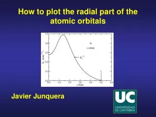
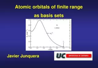
Numerical atomic orbitals Numerical solutionof the Kohn-Sham Hamiltonian for theisolated pseudoatomwith thesame approximations(xc,pseudos) as for the condensed system This equation is solved in a logarithmic grid using the Numerov method Dense close at the origin where atomic quantities oscillates wildly Light far away from the origin where atomic quantities change smoothly
Atomic orbitals: Main features that characterize the basis s Radial part: degree of freedom to play with Spherical harmonics: well defined (fixed) objects p d f Size:Number of atomic orbitals per atom Range:Spatial extension of the orbitals Shape:of the radial part
Size (number of basis set per atom) Quick exploratorycalculations Highly convergedcalculations Minimal basis set (single-ζ; SZ) Multiple-ζ + Polarization + Diffuse orbitals Depending on the required accuracy and available computational power + Basis optimization
Converging the basis size:from quick and dirty to highly converged calculations Examples of minimal basis-set: l = 0 (s) l = 1 (p) Si atomic configuration:1s2 2s2 2p63s2 3p2 m = 0 m = -1 m = 0 m = +1 valence core • Single- (minimal orSZ) • One single radial function per angular • momentum shell occupied in the free–atom 4 atomic orbitals per Si atom (pictures courtesy of Victor Luaña)
Converging the basis size:from quick and dirty to highly converged calculations Examples of minimal basis-set: Fe atomic configuration:1s2 2s2 2p6 3s2 3p6 4s2 3d6 core valence • Single- (minimal orSZ) • One single radial function per angular • momentum shell occupied in the free–atom l = 0 (s) l = 2 (d) m = 0 m = -2 m = -1 m = 0 m = +1 m = +2 6 atomic orbitals per Fe atom (pictures courtesy of Victor Luaña)
Converging the basis size:from quick and dirty to highly converged calculations • Radialflexibilization: • Add more than one radial function within the same angular momentum than SZ • Multiple- • Single- (minimal orSZ) • One single radial function per angular • momentum shell occupied in the free–atom Improving the quality
The optimal atomic orbitals are environment dependent H H R 0 (He atom) R (H atom) R r Basis set generated for isolated atoms… …but used in molecules or condensed systems Add flexibility to the basis to adjust to different configurations
Schemes to generate multiple- basis setsUse pseudopotential eigenfunctions with increasing number of nodes Advantages Orthogonal Asymptotically complete Disadvantages Excited states of the pseudopotentials, usually unbound Efficient depends on localization radii Availables in Siesta: PAO.BasisType Nodes T. Ozaki et al., Phys. Rev. B 69, 195113 (2004) http://www.openmx-square.org/
Schemes to generate multiple- basis setsChemical hardness: use derivatives with respect to the charge of the atoms Advantages Orthogonal It does not depend on any variational parameter Disadvantages Range of second- equals the range of the first- function G. Lippert et al., J. Phys. Chem. 100, 6231 (1996) http://cp2k.berlios.de/
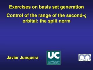
Default mechanism to generate multiple- in SIESTA: “Split-valence” method Starting from the function we want to suplement
Default mechanism to generate multiple- in SIESTA: “Split-valence” method The second- function reproduces the tail of the of the first- outside a radius rm
Default mechanism to generate multiple- in SIESTA: “Split-valence” method And continuous smoothly towards the origin as (two parameters: the second- and its first derivative continuous at rm
Default mechanism to generate multiple- in SIESTA: “Split-valence” method The same Hilbert space can be expanded if we use the difference, with the advantage that now the second- vanishes at rm (more efficient)
Default mechanism to generate multiple- in SIESTA: “Split-valence” method Finally, the second- is normalized rm controlled with PAO.SplitNorm (typical value 0.15)
Both split valence andchemical hardness methods provides similar shapes for the second- function Split valence double- has been orthonormalized to first- orbital SV: higher efficiency(radius of second- can be restricted to the inner matching radius) Chemical hardeness Split valence Gaussians E. Anglada, J. Junquera, J. M. Soler, E. Artacho, Phys. Rev. B 66, 205101 (2002)
Converging the basis size:from quick and dirty to highly converged calculations • Radialflexibilization: • Add more than one radial function within the same angular momentum than SZ • Multiple- • Angular flexibilization: • Add shells of different atomic symmetry (different l) • Polarization • Single- (minimal orSZ) • One single radial function per angular • momentum shell occupied in the free–atom Improving the quality
Example of adding angular flexibility to an atomPolarizing the Si basis set l = 0 (s) l = 1 (p) Si atomic configuration:1s2 2s2 2p63s2 3p2 m = 0 m = -1 m = 0 m = +1 valence core m = -2 m = -1 m = 0 m = +1 m = +2 Polarize: add l = 2 (d) shell New orbitals directed in different directions with respect the original basis
Two different ways of generate polarization orbitals Perturbative polarization Apply a small electric field to the orbital we want to polarize E s+p s Si 3d orbitals E. Artacho et al., Phys. Stat. Sol. (b), 215, 809 (1999)
Two different ways of generate polarization orbitals Atomic polarization Solve Schrödinger equation for higher angular momentum unbound in the free atom require short cut offs Perturbative polarization Apply a small electric field to the orbital we want to polarize E s+p s Si 3d orbitals E. Artacho et al., Phys. Stat. Sol. (b), 215, 809 (1999)
Improving the quality of the basis more atomic orbitals per atom
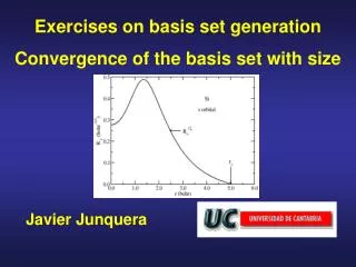
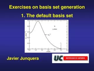
Convergence as a function of the size of the basis set: Bulk Si Cohesion curves PW and NAO convergence Atomic orbitals show nice convergence with respect the size Polarization orbitals very important for convergence (more than multiple-) Double- plus polarization equivalent to a PW basis set of 26 Ry
Convergence as a function of the size of the basis set: Bulk Si SZ DZ TZ SZP DZP TZP TZDP PW APW Exp a (Å) 5.52 5.46 5.45 5.42 5.39 5.39 5.39 5.38 5.41 5.43 B (GPa) 89 96 98 98 97 97 96 96 96 98.8 Ec (eV) 4.72 4.84 4.91 5.23 5.33 5.34 5.34 5.37 5.28 4.63 SZ = single- DZ= doble- TZ=triple- P=Polarized DP=Doble- polarized PW: Converged Plane Waves (50 Ry) APW: Augmented Plane Waves A DZP basis set introduces the same deviations as the ones due to the DFT or the pseudopotential approaches
Range: the spatial extension of the atomic orbitals If the two orbitals are sufficiently far away = 0 = 0 Order(N) methods locality, that is, a finite range for matrix and overlap matrices Neglect interactions: Below a tolerance Beyond a given scope of neighbours Difficulty: introduce numerical instabilities for high tolerances. Strictly localized atomic orbitals: Vanishes beyond a given cutoff radius O. Sankey and D. Niklewski, PRB 40, 3979 (89) Difficulty:accuracy and computational efficiencydepend on the range of the basis orbitals How to define all the rc in a balance way?
How to control the range of the orbitals in a balanced way: the energy shift Particle in a confinement potential: Imposing a finite + Continuous function and first derivative E is quantized (not all values allowed) Increasing E has a node and tends to - when x - Complement M III “Quantum Mechanics”, C. Cohen-Tannoudji et al.
How to control de range of the orbitals in a balanced way: the energy shift Energy increase Energy shift PAO.EnergyShift (energy) Cutoff radius, rc, = position where each orbital has the node A single parameter for all cutoff radii The larger the Energy shift, the shorter the rc’s Typical values: 100-200 meV E. Artacho et al. Phys. Stat. Solidi (b) 215, 809 (1999)
Convergence with the range More efficient More accurate Bulk Si equal s, p orbitals radii J. Soler et al., J. Phys: Condens. Matter, 14, 2745 (2002)
The range and shape might be also controlled by an extra charge and/or by a confinement potential Extra charge Q Orbitals in anions tend to be more delocalized Orbitals in cations tend to be more localized (For instance, this parameter might be important in some oxides) Confinement potentials Solve the Schrödinger equation for the isolated atom inside an confinement potential
Different proposals for the confinement potentials: Hard confinement a Determined by the energy shift Fireball O. F. Sankey and D. J. Niklewski, Phys. Rev. B 40, 3979 (89) The default in SIESTA Advantages: empirically, it works very nice Pitfall: produces orbitals with first derivative discontinuous at rc problem when combined with numerical grids.
Different proposals for the confinement potentials: Polynomials n = 2 [D. Porezag et al, PRB 51, 12947 (1995) ] n = 6 [ A. P. Horsfield, PRB 56, 6594 (1997) ) Advantages: orbital continuous with all the derivatives continuos Pitfall: no radius where the orbitals is strictly zero not zero in the core regions
Different proposals for the confinement potentials: Direct modification of the wave function S. D. Kenny et al., Phys. Rev. B 62, 4899 (2000) C. Elsaesser et al. J. Phys. Condens. Matter 2, 4371 (1990) Advantages: strict localization beyond rc Pitfall: bump when is large and rc is small
Different proposals for the confinement potentials: Soft-confinement potential Available in SIESTA J. Junquera et al., Phys. Rev. B 64, 235111 (2001) Advantages: orbital continuous with all the derivatives continuos diverges at rc (orbital exactly vanishes there) zero at the core region Pitfall: two new parameters to play with, more exploratory calculations
How to introduce the basis set in SIESTA Effort on defining a systematic with minimum parameters If nothing is specified: default Default value Basis size: PAO.BasisSize DZP Range of first-zeta: PAO.EnergyShift 0.02 Ry Second-zeta: PAO.BasisType Split Range of second-zeta: PAO.SplitNorm 0.15 Confinement: Hard well Good basis set in terms of accuracy versus efficiency