Javier Junquera
Molecular dynamics in different ensembles. Javier Junquera. Equations of motion for atomic systems. Classical equation of motion for a system of molecules interacting via a potential. The most fundamental form : the Lagrangian equation of motion.

Javier Junquera
E N D
Presentation Transcript
Molecular dynamics in different ensembles Javier Junquera
Equations of motion for atomic systems Classicalequation of motionfor a system of moleculesinteractingvia a potential Themost fundamental form: theLagrangianequation of motion WheretheLagrangianfunctionisdefined in terms of thekinetic and potentialenergies, and isconsideredto be a function of thegeneralizedcoordinates and their time derivatives
Equations of motion for atomic systems in cartesian coordinates Classicalequation of motionfor a system of moleculesinteractingvia a potential Ifweconsider a system of atomswithCartesiancoordinates , and the usual definitions of thekinetic and potentialenergies Then, theequation of motiontransformsinto whereisthemass of atom and theforceonthatatomisgivenby
Equations of motion for atomic systems in cartesian coordinates Classicalequation of motionfor a system of moleculesinteractingvia a potential Thisequationalsoapliestothe center of massmotion of a molecule, withtheforcebeginthe total externalforceactingonit
Hamilton’s equation of motion in cartesian coordinates For a derivation of theseexpressions, readGoldstein, Chapter 8
Hamilton or Lagrange equations of motion Lagrange’sequation Hamilton’sequations To compute the center of masstrajectoriesinvolvessolving… A system of 3Nsecondorderdifferentialequations Oranequivalent set of 6Nfirst-orderdifferentialequations
Hamilton or Lagrange equations of motion Lagrange’sequation Hamilton’sequations To compute the center of masstrajectoriesinvolvessolving… A system of 3Nsecondorderdifferentialequations Oranequivalent set of 6Nfirst-orderdifferentialequations
Conservation laws Assumingthat and do notdependexplicitlyon time, so that Essentialcondition: No explicitly time dependentorvelocitydependentforceacting Then, the total derivative of theHamiltonianwithrespectto time FromtheHamilton’sequation of motion TheHamiltonianis a constant of motion Independent of theexistence of anexternalpotential
The equations are time reversible Bychangingthesigns of allthevelocities and momenta, wewill cause themoleculestoretracetheirtrajectories. Iftheequations of motion are solvedcorrectly, thecomputer-generatedtrajectorieswillalsohavethisproperty
Standard method to solve ordinary differential equations: the finite difference approach Given molecular positions, velocities, and otherdynamicinformation at a time Notes: Theequations are solvedon a stepbystepbasis Thechoice of the time intervalwilldependonthemethod of solution, butwill be significantlysmallerthanthetypical time takenfor a moleculetotravelitsownlength Weattempttoobtainthe position, velocities, etc. at a later time , to a sufficientdegree of accuracy
Many different algorithms within the finite different methodology Predictor-corrector algorithm
If the classical trajectory is continuous, then an estimate of the positions, velocities, accelerations at can be obtained by a Taylor expansion about time Westorefour “vectors” per atom: stands for “predicted” stands forthe complete set of positions stands forthe complete set of velocities stands forthe complete set of accelerations stands forthe complete set of thirdderivatives of the position
If the classical trajectory is continuous, then an estimate of the positions, velocities, accelerations at can be obtained by a Taylor expansion about time stands for “predicted” Ifwetruncatetheexpansionretainingthetermsgivenabove Wehaveachievedourgoal of approximatelyadvancingthevalues of thedynamicalquantitesfromone time steptothenext Wewillnotgeneratecorrecttrajectories as time advancesbecausewehavenotintroducedtheequations of motion
The equations of motion are introduced through the correction step From the new predicted positions we can compute the forces at time , and hence correct accelerations The correct accelerations can be compared with the predicted accelerations to estimate the size of the error in the prediction step Thiserrors, and theresults of the predictor step, are fedintothe corrector step These positions, velocities, etc. are betterapproximationstothe true positions, velocities, etc.
“Best choices” (leading to optimum stability and accuracy of the trajectories) for the coefficients discussed by Gear Differentvalues of thecoefficients are requiredifweinclude more (orfewer) position derivatives in ourscheme Thecoefficientsalsodependupontheorder of thedifferentialequationbeingsolved (secondorder in our case) Ifthe positions, velocities, accelerations, etc. are unscaled, factorsinvolvingthe time scaled are required (seealgorithmbelow)
Implementation of Gear’s predictor-corrector algorithm The predictor part
Implementation of Gear’s predictor-corrector algorithm The corrector part
The corrector step might be iterated till convergence New correct accelerations are computed from the positions and compared with the current values of , so as to further refine the positions, velocities, etc. In many applications this iteration is key to obtaining an accurate solution However, each iteration requires a computation of the forces from particle positions (the most time-consuming part of the simulation) A large number of corrector iterations would be very expensive. Normally one (occasionally two) corrector steps are carried out
General step of a stepwise Molecular Dynamics simulation Predict the positions, velocities, accelerations, etc. at a time , using the current values of these quantities Evaluate the forces, and hence the accelerations from the new positions Correct the predicted positions, velocities, accelerations, etc. using the new accelerations Calculate any variable of interest, such as the energy, virial, order parameters, ready for the accumulation of time averages, before returning to the first point for the next step
Desirable qualities for a successful simulation algorithm Itshould be fast and requirelittlememory Sincethemost time consumingpartistheevaluation of theforce, therawspeed of theintegrationalgorithmisnot so important It should permit the use of long time step Far more importanttoemploy a long time step. In thisway, a givenperiod of simulation time can be covered in a modestnumber of steps Itshouldduplicatetheclassicaltrajectory as closely as possible It should satisfy the known conservation laws for energy and momentum, and be time reversible It should be simple in form and easy to program Involvethestorage of only a fewcoordinates, velocitites,…
Desirable qualities for a successful simulation algorithm Itshould be fast and requirelittlememory Sincethemost time consumingpartistheevaluation of theforce, therawspeed of theintegrationalgorithmisnot so important It should permit the use of long time step Far more importanttoemploy a long time step. In thisway, a givenperiod of simulation time can be covered in a modestnumber of steps Itshouldduplicatetheclassicaltrajectory as closely as possible It should satisfy the known conservation laws for energy and momentum, and be time reversible It should be simple in form and easy to program Involvethestorage of only a fewcoordinates, velocitites,…
The accuracy and stability of a simulation algorithm may be tested comparing the result with analytical simple models (Harmonic oscillator, for instance) Anyapproximatemethod of solutionwilldutifullyfollowtheclassicaltrajectoryindefinetely Small differences in theinitialconditions Small numericalerrors Anysmallperturbation, eventhetiny error associatedwithfiniteprecisionarithmetic, willtendto cause a computer-generatedtrajectoryto diverge fromthe true classicaltrajectorywithwhichitisinitiallycoincident Anytwotrajectorieswhich are initiallyveryclosewilleventually diverge fromoneanotherexponentiallywith time
The accuracy and stability of a simulation algorithm may be tested comparing the result with analytical simple models (Harmonic oscillator, for instance) Anyapproximatemethod of solutionwilldutifullyfollowtheclassicaltrajectoryindefinetely Divergence of trajectories in molecular dynamics As the time proceeds, othermechanicalquantitesbecomestatisticallyuncorrelated Moleculesperturbedfromtheinitial positions at t=0 by Small differences in theinitialconditions Anytwotrajectorieswhich are initiallyveryclosewilleventually diverge fromoneanotherexponentiallywith time Reference simulation Perturbedsimulation
The accuracy and stability of a simulation algorithm may be tested comparing the result with analytical simple models (Harmonic oscillator, for instance) Anyapproximatemethod of solutionwilldutifullyfollowtheclassicaltrajectoryindefinetely No integrationalgorithmwillprovideanessentiallyexactsolutionfor a verylong time Butthisisnotreallyrequired… Whatweneed are: Exactsolutions of theequations of motionfor times comparable withthecorrelation times of interest, so we can calculate time correlationfunctions Themethod has togeneratestatessampledfromthemicrocanonicalensemble. Theemphasis has to be giventotheenergyconservation. Theparticlestrajectoriesmuststayontheappropriateconstant-energyhypersurfaces in phasespacetogeneratecorrectensembleaverages
Energy conservation is degraded as time step is increased ECONOMY ACCURACY Allsimulationsinvolve a trade-off between A good algorithm permits a large time step to be used while preserving acceptable energy conservation
Parameters that determine the size of • Shape of thepotentialenergy curves • Typical particle velocities Shorter time steps are used at high-temperatures, for light molecules, and forrapidlyvaryingpotentialfunctions
The Verlet algorithm method of integrating the equations of motion: description of the algorithm Method based on: - the positions - the accelerations - the positions from the previous step Direct solution of the second-order equations A Taylor expansion of the positions around t Adding the two equations
The Verlet algorithm method of integrating the equations of motion: some remarks Remark 1 The velocities are not needed to compute the trajectories, but they are useful for estimating the kinetic energy (and the total energy). They can be computed a posteriori using [ can only be computed once is known] Remark 2 Whereas the errors to compute the positions are of the order of The velocities are subject to errors of the order of
The Verlet algorithm method of integrating the equations of motion: some remarks Remark 3 The Verlet algorithm is properly centered: and play symmetrical roles. The Verlet algorithm is time reversible Remark 4 Theadvancement of positions takes place allin onego, ratherthan in twostages as in the predictor-corrector algorithm.
The Verlet algorithm method of integrating the equations of motion: some remarks • Letusassumethatwehaveavailablecurrent (RX) and old (RXOLD). • Thecurrentaccelerations (AX) are evaluated in theforceloop as usual. • Then, thecoordinates are advanced in thefollowingway
The Verlet algorithm method of integrating the equations of motion: some remarks • Letusassumethatwehaveavailablecurrent (RX) and old (RXOLD). • Thecurrentaccelerations (AX) are evaluated in theforceloop as usual. • Then, thecoordinates are advanced in thefollowingway Use of temporary variables (RXNEWI) tostorethe new positions. Thisisnecessarybecausethecurrentvaluesmust be transferredtothe “old” positions beforebeingoverwrittenwiththe new variables. Thecalculation of kineticenergy (SUMVSQ) and the total linear momentum (SUMVX) isincluded in theloop, sincethisistheonlymoment at which and are known.
The Verlet algorithm method of integrating the equations of motion: overall scheme …and we repeat the process computing the forces (and therefore the accelerations at ) Known the positions at t, we compute the forces (and therefore the accelerations at t) Then, we apply the Verlet algorithm equations to compute the new positions
The Verlet algorithm method of integrating the equations of motion: advantages The Verlet algorithm requires 9N words of storage (RX, RXOLD, AX, and the corresponding for the y and z coordinates) The algorithm is exactly reversible in time, and, given conservative forces, is guaranteed to conserve linear momentum and energy The method has been shown to have excellent energy conserving properties even in long time steps
The Verlet algorithm method of integrating the equations of motion: drawbacks A small term of order … …is added to a difference of large terms, of order The handling of velocities is rather awkward It may introduce some numerical imprecision
The half-step “leap-frog” scheme tackles the deficiencies of the Verlet algorithm Method based on: - the positions - the accelerations - the mid-step velocities Algorithm
Scheme of the half-step “leap-frog” algorithm …and we repeat the process computing the new velocities at The velocity equation is implemented first, and the velocities leap over the coordinates Then, we apply the leap-frog algorithm to compute the new positions Known the new positions, we compute the forces and therefore the accelerations… At a given t, we can compute the velocities, required to calculate the total energy
The half-step “leap-frog” scheme: advantages and disadvantages Advantages Elimination of velocities from the leap-frog equations, the method is algebraically equivalent to Verlet’s algorithm At no stage do we take the difference of two large quantities to obtain a small value, minimizing loss of precision on a computer Disadvantages Still do not handle the velocities in a complete satisfactory way
The velocity Verlet algorithm: algorithm and advantages Algorithm Advantages Stores the positions, velocities, and accelerations at the same time t Minimizes rounds-off errors The Verlet algorithm can be recovered by eliminating the velocities
Scheme of the velocity Verlet algorithm The velocities at mid step are computed using Known the new positions, we compute the forces and therefore the accelerations at time The velocity move is completed Known the positions, velocities and accelerations at t, we compute the new positions at At thispointthekineticenergyisavailable Thepotentialenergy has beenevaluated in theforceloop
The velocity Verlet algorithm: advantages Themethoduses 9Nwords of storage Numericallystable Very simple
Is the code working?: First check: the conservation laws are properly obeyed Theenergyshould be “constant” In fact, smallchanges in energywilloccur. For simple Lennard-Jones system, fluctuations of 1 part in 104 are generallyconsideredto be acceptable Energyfluctuationsmight be reducedbydecreasingthe time step Suggestiontocheckaccuracy: Several short runsshould be undertaken, eachstartingfromthesameinitialconfiguration and coveringthesame total time Eachrunshouldemploy a different time step (differentnumber of steps ) Theroot mean squarefluctuationsforeachrunshould be calculated
Is the code working?: First check: the conservation laws are properly obeyed Suggestiontocheckaccuracy: Theroot mean squarefluctuationsforeachrunshould be calculated Several short runsshould be undertaken, eachstartingfromthesameinitialconfiguration and coveringthesame total time Iftheprogramisfunctioningcorrectly, theVerletalgorithmshouldgive RMS fluctuationsthat are accuratelyproportionalto Eachrunshouldemploy a different time step (differentnumber of steps )