Correcting for the lifetime dependent cuts
120 likes | 270 Vues
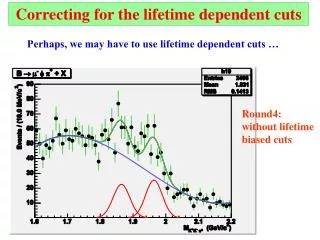
Correcting for the lifetime dependent cuts. Perhaps, we may have to use lifetime dependent cuts …. Round4: without lifetime biased cuts. Without biases, lifetime distribution ~ e t/ convoluted with a Gaussian in real life (RECO) due to finite detector resolution

Correcting for the lifetime dependent cuts
E N D
Presentation Transcript
Correcting for the lifetime dependent cuts Perhaps, we may have to use lifetime dependent cuts … Round4: without lifetime biased cuts
Without biases, lifetime distribution ~ et/ • convoluted with a Gaussian in real life (RECO) due to finite detector resolution • With lifetime-dependent/biased cuts, it is no longer et/, but (say) f(t) which is what I am after. • Goal is to find f(t) from the Monte Carlo using the “Truth” information which does not suffer from detector resolution. • Reco-ed tracks are matched with the MC: • |pT| < 0.5, ||< 0.02, ||< 0.02
I’ve taken Wendy’s code (on top of the bmixing_reco) to grab the necessary Monte Carlo information • it deals with the Bs mixing information correctly • I’ve also used Vivek’s lifetime-dependent or independent cuts: round4
Biased cuts: • Imp()/ > 9 || Imp()/ > 9 || Imp(K)/ > 9 ; • Imp()/ alone > 2 • If ( Lxy(D) < Lxy(B) ) |Imp(BD)/| < 3 • cos(D,B) > 0.85; COLL > 0. Unbiased cuts: • pT() > 1.5 ; pT() > 0.7; pT(K) > 0.7 • Ptot(B) > 8 ; Ptot() > 3 ; Prel() > 1 • 1.006 < M() < 1.032 GeV • Helicity (K,D) > 0.5
Only MC “Truth” information VPDL ~ Lxy(B)*M(B)/pT(Ds) Without cuts x–axes in cm With cuts
Only MC “Truth” information Lifetime ~ Lxy(B)*M(B)/pT(B) Without cuts x–axes in cm With cuts
For now (at least), we consider the ratios of lifetime with and without certain cuts. For now (at least), we look at the ratio of the lifetimes with and without certain cuts. x–axes in cm
Thinking … • f(t) ~ ( p2 - p0ep1t ) et/ • With no biased cuts, reconstructed lifetime distribution in data ~ EG dt where E ~ et/ when t0; otherwise E=0; • With biased cuts, the distribution is ~ E( p2 - p0ep1t) G dt
Fitting E( p2 - p0ep1 t ) G dtagainst the reconstructed VPDL when all the cuts are applied. Fitting EG dt against the reconstructed VPDL when there is no cut applied. x–axes in cm
To do … • The 2 Gaussian ’s are quite different in the 2 fits • Need to understand what it is going on … I’ve checked by • fitting the 2 convoluted functions on the MC “Truth” lifetime and I do get very small Gaussian . • fitting the 2 convoluted on the toy MC distributions to get the right sigma that I put in. • Tried adding mass cuts/separating events into 2 groups … don’t help
Backup Slides VPDL resolution One Gaussian fit Two Gaussian fit x–axes in cm