Download
1 / 52
520 likes | 613 Vues
Learn the mathematical formulation and importance of knowing the demand curve in online posted-price auctions. Explore regret bounds and strategies of informed vs. uninformed sellers.

E N D
The Value of Knowing a Demand Curve:Regret Bounds for Online Posted-Price Auctions Bobby Kleinberg and Tom Leighton
Introduction • How do we measure the value of knowing the demand curve for a good?
Introduction • How do we measure the value of knowing the demand curve for a good? • Mathematical formulation: What is the difference in expected revenue between • an informed seller who knows the demand curve, and • an uninformed seller using an adaptive pricing strategy … assuming both pursue the optimal strategy.
Online Posted-Price Auctions • 1 seller, n buyers, each wants one item. • Buyers interact with seller one at a time. • Transaction: • Seller posts price.
6¢ Online Posted-Price Auctions • 1 seller, n buyers, each wants one item. • Buyers interact with seller one at a time. • Transaction: • Seller posts price. • Buyer arrives.
6¢ Online Posted-Price Auctions • 1 seller, n buyers, each wants one item. • Buyers interact with seller one at a time. • Transaction: • Seller posts price. • Buyer arrives. • Buyer gives YES/NO response. YES
Online Posted-Price Auctions • 1 seller, n buyers, each wants one item. • Buyers interact with seller one at a time. • Transaction: • Seller posts price. • Buyer arrives. • Buyer gives YES/NO response. • Seller may update price YES 10¢ after each transaction.
Online Posted-Price Auctions • A natural transaction model for many forms of commerce, including web commerce. (Our motivation came from ticketmaster.com.) 10¢
Online Posted-Price Auctions • A natural transaction model for many forms of commerce, including web commerce. (Our motivation came from ticketmaster.com.) • Clearly strategyproof, since agents’ strategic behavior is limited to their YES/NO responses. 10¢
Informed Informed vs. Uninformed Sellers Uninformed
Uninformed Informed Informed vs. Uninformed Sellers
Uninformed Informed Informed vs. Uninformed Sellers
Uninformed Informed Informed vs. Uninformed Sellers
Uninformed Informed Informed vs. Uninformed Sellers
Uninformed Informed Informed vs. Uninformed Sellers
Uninformed Informed Informed vs. Uninformed Sellers
Uninformed Informed Informed vs. Uninformed Sellers
Uninformed Informed Informed vs. Uninformed Sellers Ex ante regret = 0.5 1.1 1.6
Uninformed Informed Informed vs. Uninformed Sellers Ex post regret = 1.0 1.1 2.1
Definition of Regret • Regret= difference in expected revenue between informed and uninformed seller. • Ex ante regret corresponds to asking,“What is the value of knowing the demand curve?” • Competitive ratio was already considered by Blum, Kumar, et al (SODA’03). They exhibited a (1+ε)-competitive pricing strategy under a mild hypothesis on the informed seller’s revenue.
3 Problem Variants • Identical valuations: All buyers have same threshold price v, which is unknown to seller. • Random valuations: Buyers are independent samples from a fixed probability distribution (demand curve) which is unknown to seller. • Worst-case valuations: Make no assumptions about buyers’ valuations, they may be chosen by an oblivious adversary. • Always assume prices are between 0 and 1.
Ex ante Ex post Regret Bounds for the Three Cases
Identical Valuations • Exponentially better than binary search!! • Equivalent to a question considered by Karp, Koutsoupias, Papadimitriou, Shenker in the context of congestion control. (KKPS, FOCS 2000). • Our lower bound settles two of their open questions.
Random Valuations 1 Demand curve: D(x) = Pr(accepting price x) D(x) 0 x 1
1 D(x) 0 x 1 Best “Informed” Strategy Expected revenue at price x: f(x) = xD(x).
1 D(x) 0 x 1 Best “Informed” Strategy If demand curve is known, best strategy is fixed price maximizing area of rectangle.
1 D(x) 0 x 1 Best “Informed” Strategy If demand curve is known, best strategy is fixed price maximizing area of rectangle. Best known uninformed strategy is based on the multi-armed bandit problem...
You are in a casino with K slot machines. Each generates random payoffs by i.i.d. sampling from an unknown distribution. The Multi-Armed Bandit Problem
You are in a casino with K slot machines. Each generates random payoffs by i.i.d. sampling from an unknown distribution. You choose a slot machine on each step and observe the payoff. The Multi-Armed Bandit Problem 0.3 0.7 0.4 0.5 0.1 0.6 0.2 0.2 0.7 0.3 0.8 0.5 0.6 0.1 0.4
You are in a casino with K slot machines. Each generates random payoffs by i.i.d. sampling from an unknown distribution. You choose a slot machine on each step and observe the payoff. Your expected payoff is compared with that of the best single slot machine. The Multi-Armed Bandit Problem 0.3 0.7 0.4 0.5 0.1 0.6 0.2 0.2 0.7 0.3 0.8 0.5 0.6 0.1 0.4
Assuming best play: Ex ante regret = θ(log n) [Lai-Robbins, 1986] Ex post regret = θ(√n) [Auer et al, 1995] Ex post bound applies even if the payoffs are adversarial rather than random. (Oblivious adversary.) The Multi-Armed Bandit Problem 0.3 0.7 0.4 0.5 0.1 0.6 0.2 0.2 0.7 0.3 0.8 0.5 0.6 0.1 0.4
Application to Online Pricing • Our problem resembles a multi-armed bandit problem with a continuum of “slot machines”, one for each price in [0,1]. • Divide [0,1] into Ksubintervals, treat them as a finite set of slot machines.
Application to Online Pricing • Our problem resembles a multi-armed bandit problem with a continuum of “slot machines”, one for each price in [0,1]. • Divide [0,1] into Ksubintervals, treat them as a finite set of slot machines. • The existing bandit algorithms have regret O(K2 log n + K-2n), provided xD(x) is smooth and has a unique global max in [0,1]. • Optimizing K yields regret O((n log n)½).
The Continuum-Armed Bandit • The continuum-armed bandit problem has algorithms with regret O(n¾), when exp. payoff depends smoothly on the action chosen.
? The Continuum-Armed Bandit • The continuum-armed bandit problem has algorithms with regret O(n¾), when exp. payoff depends smoothly on the action chosen. • But: Best-known lower bound on regret was Ω(log n) coming from the finite-armed case.
The Continuum-Armed Bandit • The continuum-armed bandit problem has algorithms with regret O(n¾), when exp. payoff depends smoothly on the action chosen. • But: Best-known lower bound on regret was Ω(log n) coming from the finite-armed case. • We prove: Ω(√n). ?
1 D(x) 0 x 1 Lower Bound: Decision Tree Setup
1 D(x) 0 x 1 Lower Bound: Decision Tree Setup 0.3 ½ ¼ ¾ ⅛ ⅜ ⅝ ⅞
1 D(x) 0 x 1 Lower Bound: Decision Tree Setup 0.2 ½ ¼ ¾ ⅛ ⅜ ⅝ ⅞
1 D(x) 0 x 1 Lower Bound: Decision Tree Setup 0.4 ½ ¼ ¾ ⅛ ⅜ ⅝ ⅞
Lower Bound: Decision Tree Setup ½ ¼ ¾ ⅛ ⅜ ⅝ ⅞
Natural idea: Lower bound on incremental regret at each level… How not to prove a lower bound! ½ ¼ ¾ ⅛ ⅜ ⅝ ⅞
Natural idea: Lower bound on incremental regret at each level… If regret is Ω(j-½) at level j, then total regret after n steps would be Ω(√n). How not to prove a lower bound! ½ 1 ¼ ¾ √½ ⅛ ⅜ ⅝ ⅞ √⅓ 1 +√½ + √⅓ + … = Ω(√n)
Natural idea: Lower bound on incremental regret at each level… If regret is Ω(j-½) at level j, then total regret after n steps would be Ω(√n). This is how lower bounds were proved for the finite-armed bandit problem, for example. How not to prove a lower bound! ½ 1 ¼ ¾ √½ ⅛ ⅜ ⅝ ⅞ √⅓ 1 +√½ + √⅓ + … = Ω(√n)
The problem: If you only want to minimize incremental regret at level j, you can typically make it O(1/j). Combining the lower bounds at each level gives only the very weak lower bound Regret = Ω(log n). How not to prove a lower bound! ½ 1 ¼ ¾ ½ ⅛ ⅜ ⅝ ⅞ ⅓ 1 +½ + ⅓ + … = Ω(log n)
How to prove a lower bound • So instead a subtler approach is required. • Must account for the cost of experimentation. • We define a measure of knowledge, KD such that regret scales at least linearly with KD. • KD = ω(√n) → TOO COSTLY • KD = o(√n) → TOO RISKY ½ ¼ ¾ ⅛ ⅜ ⅝ ⅞
Discussion of lower bound • Our lower bound doesn’t rely on a contrived demand curve. In fact, we show that it holds for almost every demand curve satisfying some “generic” axioms. (e.g. smoothness)
Discussion of lower bound • Our lower bound doesn’t rely on a contrived demand curve. In fact, we show that it holds for almost every demand curve satisfying some “generic” axioms. (e.g. smoothness) • The definition of KD is quite subtle. This is the hard part of the proof.
Discussion of lower bound • Our lower bound doesn’t rely on a contrived demand curve. In fact, we show that it holds for almost every demand curve satisfying some “generic” axioms. (e.g. smoothness) • The definition of KD is quite subtle. This is the hard part of the proof. • An ex post lower bound of Ω(√n) is easy. The difficulty is solely in strengthening it to an ex ante lower bound.
Open Problems • Close the log-factor gaps in random and worst-case models.