UCN transport and NN experiments
60 likes | 212 Vues
UCN transport and NN experiments. R. Young and B. Wehring NCState University. The geometry:. How do we model transport?. Transport Data: Where Does It Come From?. Raw Data:. TOF – proton start, detector stop. LANSCE Prototype Source:. Modeling strategy, model date using fit parameters:

UCN transport and NN experiments
E N D
Presentation Transcript
UCN transport and NN experiments R. Young and B. Wehring NCState University
The geometry: How do we model transport?
Transport Data: Where Does It Come From? Raw Data: TOF – proton start, detector stop LANSCE Prototype Source: • Modeling strategy, model date using fit parameters: • specularity (TOF very sensitive) • loss per bounce, shape of SD2 and UCN lifetime in SD2 (use “bottle lifetime between source and valve A) For lifetime: study thin films so mfp in SD2 not important
Prototype Results Specularity: average probability that a reflection will be mirror-like Loss per bounce: average probability that UCN will be absorbed or upscattered during a collision • Specularity: 97.5% ( roughly 2% uncertainty) agrees with measurements of straight and curved guides we have performed at ILL • Loss per bounce: .0025 conservative, set by 58Ni bottle lifetimes and source data 58Ni/Mo coated guides (approx. 305 neV) PLD diamond coatings (250 - 300 neV, with 300 neV measured for at SPEAR) • Specularity: >99% (data obtained at ILL recently for drawn quartz tubes) • Loss per bounce < .00016 (data from ILL expts – negligible for our purposes)
The Monte Carlo • Runge-Kutta numerical integration • Gravity, magnetic fields (if needed), and wall reflections • Non-specular reflections via various models (Gaussian, isotropic and Lambertian—(from Golub, Richardson, Lamoreaux) • Spin dynamics if needed (depolarization on surfaces and spin dynamics in rf fields) (future effort: n-n phase evolution) • Assume n annihilated on each collision
Preliminary results for base case (det eff = 1): • A possible base case: NCState geometry, 4 cm thick SD2, 18 cm guides, .050s SD2 lifetime, a UCN energy cutoff of 430 neV initally Primary flux: 6.0 x 10⁷ (below 305 neV) Box loading efficiency: 20 –32% Best case: diffuse walls, specular floor 3.5x10^9 discovery pot. 325 s avg. residency • Straightforward gains: Source thickness x2 (see Serebrov’s geom): x 2 Source lifetime .075s +10% Running time: 4 years (“real”) • Speculative gains: Multiphonon: x1.5(?) Coherent amplification: x2 (?) Solid Oxygen: x5 (?) 5.5 – 7 x 10⁹ Various diffuse regions, wall potentials, same “best” case as above