LR for Packing problems
LR for Packing problems. Reuven Bar-Yehuda www.cs.technion.ac.il/~reuven. The Local-Ratio Technique: Basic definitions . Given a profit [penalty] vector p. Maximize[Minimize] p·x Subject to: feasibility constraints F(x) x is r-approximation if F(x) and p·x [] r · p·x*

LR for Packing problems
E N D
Presentation Transcript
LR forPacking problems Reuven Bar-Yehuda www.cs.technion.ac.il/~reuven
The Local-Ratio Technique: Basic definitions • Given a profit [penalty] vector p. • Maximize[Minimize]p·x • Subject to: feasibility constraints F(x) • x isr-approximationif F(x) and p·x []r·p·x* • An algorithm is r-approximationif for any p, F • it returns an r-approximation
The Local-Ratio Theorem: • xis an r-approximation with respect to p1 • xis an r-approximation with respect to p- p1 • • xis an r-approximation with respect to p • Proof: (For maximization) • p1 · x r ×p1* • p2 · x r ×p2* • • p · x r ×( p1*+ p2*) • r ×(p1 + p2 )*
Special case: Optimization is 1-approximation • xis an optimum with respect to p1 • xis an optimum with respect to p- p1 • xis an optimum with respect to p
A Local-Ratio Schema for Maximization[Minimization] problems: • Algorithm r-ApproxMax[Min]( Set, p ) • If Set = Φ then returnΦ ; • If I Setp(I) 0 then returnr-ApproxMax( Set-{I}, p ) ; • [If I Setp(I)=0 then return {I} r-ApproxMin( Set-{I}, p ) ;] • Define “good” p1 ; • REC = r-ApproxMax[Min]( S, p- p1) ; • If REC is not an r-approximation w.r.t. p1 then “fix it”; • return REC;
Maximum Independent Set in Interval Graphs • Activity9 • Activity8 • Activity7 • Activity6 • Activity5 • Activity4 • Activity3 • Activity2 • Activity1 • time • Maximize s.t.For each instance I: • For each time t:
Maximum Independent Set in Interval Graphs: How to select P1 to get optimization? • P1=0 • Activity9 • Activity8 • Activity7 • Activity6 • Activity5 • Activity4 • Activity3 • Activity2 • Activity1 Î • time • Let Î be an interval that ends first; • 1 if I in conflict with Î • For all intervals I define: p1(I) = • 0 else • For every feasible x: p1 ·x 1 • Every Î-maximal is optimal. • For every Î-maximal x: p1 ·x 1 • P1=1 • P1=0 • P1=0 • P1=0 • P1=1 • P1=0 • P1=1 • P1=1
Maximum Independent Set in Interval Graphs: An Optimization Algorithm • P1=P(Î ) • Activity9 • Activity8 • Activity7 • Activity6 • Activity5 • Activity4 • Activity3 • Activity2 • Activity1 Î • time • Algorithm MaxIS( S, p ) • If S = Φ then returnΦ ; • If ISp(I) 0 then returnMaxIS( S - {I}, p); • Let ÎS that ends first; • IS define: p1(I) = p(Î) (I in conflict with Î) ; • IS = MaxIS( S, p- p1) ; • If IS is Î-maximal then returnIS else return IS {Î}; • P1=0 • P1=0 • P1=0 • P1=0 • P1=P(Î ) • P1=0 • P1=P(Î ) • P1=P(Î )
Maximum Independent Set in Interval Graphs: Running Example • P(I5) = 3 -4 • P(I6) = 6 -4 -2 • P(I3) = 5 -5 • P(I2) = 3 -5 • P(I1) = 5 -5 • P(I4) = 9 -5 -4 • -4 • -5 • -2
Bar-Noy, Guha, Naor and Schieber STOC 99: 1/2 LP • Berman, DasGupta, STOC 00: 1/2 • This Talk, STOC 00(Independent) 1/2 Single Machine Scheduling : • Activity9 • Activity8 • Activity7 • Activity6 • Activity5 • Activity4 • Activity3 • Activity2 • Activity1 ????????????? • time • Maximize s.t.For each instance I: • For each time t: • For each activity A:
Single Machine Scheduling: How to select P1 to get ½-approximation ? • P1=1 • P1=0 • Activity9 • Activity8 • Activity7 • Activity6 • Activity5 • Activity4 • Activity3 • Activity2 • Activity1 Î • time • Let Î be an interval that ends first; • 1 if I in conflict with Î • For all intervals I define: p1(I) = • 0 else • For every feasible x: p1 ·x 2 • Every Î-maximal is 1/2-approximation • For every Î-maximal x: p1 ·x 1 • P1=0 • P1=1 • P1=0 • P1=0 • P1=0 • P1=0 • P1=0 • P1=0 • P1=1 • P1=0 • P1=1 • P1=0 • P1=0 • P1=1 • P1=1 • P1=1 • P1=1 • P1=1
Single Machine Scheduling: The ½-approximation Algorithm • Activity9 • Activity8 • Activity7 • Activity6 • Activity5 • Activity4 • Activity3 • Activity2 • Activity1 Î • time • Algorithm MaxIS( S, p ) • If S = Φ then returnΦ ; • If ISp(I) 0 then returnMaxIS( S - {I}, p); • Let ÎS that ends first; • IS define: p1(I) = p(Î) (I in conflict with Î) ; • IS = MaxIS( S, p- p1) ; • If IS is Î-maximal then returnIS else return IS {Î};
Albers, Arora, Khanna SODA 99: O(1) |Ai|=1* • Uma, Phillips, Wein SODA 00: 1/4 LP. • This Talk 1/3 for w 1/2 and 1/5 for w 1 Bandwidth Allocation • Activity9 • Activity8 • Activity7 • Activity6 • Activity5 • Activity4 • Activity3 • Activity2 • Activity1 I w(I) • s(I) e(I) time • Maximize s.t.For each instance I: • For each time t: • For each activity A:
Bandwidth Allocation • Activity 9 • Activity 8 • Activity 7 • Activity 6 • Activity 5 • Activity 4 • Activity 3 • Activity 2 • Activity 1 • time • Bandwidth • time
Bandwidth Allocation for w 1/2 How to select P1 to get 1/3-approximation? • Activity9 • Activity8 Î • Activity7 • Activity6 • Activity5 • Activity4 • Activity3 • Activity2 • Activity1 I w(I) • s(I) e(I) time • 1if I in the same activity of Î • For all intervals I define: p1(I) = 2*w(I)if I in time conflict with Î • 0 else • For every feasible x: p1 ·x 3 • Every Î-maximal is 1/3-approximation • For every Î-maximal x: p1 ·x 1
Bandwidth Allocation The 1/5-approximation for any w 1 • Activity9 • Activity8 w > ½ • Activity7 w > ½ w > ½ • Activity6 • Activity5 w > ½ • Activity4 • Activity3 w > ½ w > ½ • Activity2 • Activity1 w > ½w > ½ w > ½ • Algorithm: • GRAY = Find 1/2-approximation for gray (w>1/2) intervals; • COLORED = Find 1/3-approximation for colored intervals • Return the one with the larger profit • Analysis: • If GRAY* 40%OPT then GRAY 1/2(40%OPT)=20%OPT else • COLORED* 60%OPT thus COLORED 1/3(60%OPT)=20%OPT
Single Machine Scheduling with Release and Deadlines • Activity 9 • Activity 8 • Activity 7 • Activity 6 • Activity 5 • Activity 4 • Activity 3 • Activity 2 • Activity 1 • time • Each job has a time window within which it can be processed.
Single Machine Scheduling with Release and Deadlines • Activity 9 • Activity 8 • Activity 7 • Activity 6 • Activity 5 • Activity 4 • Activity 3 • Activity 2 • Activity 1
Continuous Scheduling • { • Single Machine Scheduling (w=1) • Bar-Noy, Guha, Naor and Schieber STOC 99: 1/3 Non Combinatorial • Berman, DasGupta STOC 00: 1/2·(1-) • This Talk, STOC 00: (Independent) 1/2·(1-) • Bandwidth AllocationUma, Phillips, Wein SODA 00: 1/6 Noncombinatorial • This Talk, STOC 00 (Independent) 1/3 ·(1-) for w 1/2 1/5 ·(1-) for w 1 • w(I) • d(I) • s(I) e(I)
Continuous Scheduling: Split and Round Profit (Loose additional (1-) factor) • If currant p(I1) original p(I1) then delete I1 • else Split I2=(s2,e2] to I21=(s2, s1+d1] and I22=(s1+d1,e2] • d(I1) • d(I2) • I11 • I12 • d(I1) • I21 • I22 • d(I2)
LP RoundingusingFractional Local Ratio Reuven Bar-Yehuda www.cs.technion.ac.il/~reuven
General framework: Given a weight vector w. Minimize [Maximize]w·x Subject to: feasibility constraints F(x) x is anr-approximationif F(x) and w·x rw·x* [w·x rw·x* ] An algorithm is anr-approximation if for any w, F it returns an r-approximation
8 12 5 20 10 6 $1 $1 $4 $1 $1 $3 15 $2 $1 Min 5xBisli+8xTea+12xWater+10xBamba+20xShampoo+15xPopcorn+6xChocolate +$4xWaterShampoo+ • • • s.t. xShampoo + xWater + xWaterShampoo 1
The generalized vertex cover problem Minimize w·x Subject to: xu + xv + xe 1 e={u,v} E x{0,1}|V|+|E|
2-Approx GVC(G,w) If E= return If e E w(e)=0 return {e}+GVC(G-e, w) If v V w(v)=0 return {v}+GVC(G-E(v), w) Let e={u,v} E s.t = min {w(u), w(v), w(e)}>0. if x{u,v,e} w1(x)= 0 else Notice:w1x 2w1x for Good(x) REC= GVC(G, w2= w-w1) Induction hyp is: w2REC 2w2x so if Good(REC):w1REC 2w1x we are done If REC-e is a cover thenREC=REC-e Return REC
“2 integral for the price of 1 fractional”: The local ratio technique for rounding Let xbe the the fractional solution Minimize w·x Subject to: xu + xv + xe 1 e=(u,v) E x[0,1]|V|+|E|
“d integral for the price of ½(d+1) fractional”:2-2/(Δ+1)-Approx GVC(G,w) If E= return If e E w(e)=0 return {e}+GVC(G-e, w) If v V w(v)=0 return {v}+GVC(G-E(v)-v, w) Let v V s.txv is minimum and Let =min(w(i) : i N[v]} if i N[v] w1(i)= 0 else Claim:w1x rΔw1x for Good(x) REC= GVC(G, w2= w-w1) Induction hyp is: w2RECrΔw2x so if Good(REC):w1RECrΔw1x we are done If REC is not a minimal cover then make REC minimal Return REC Min xv
“d integral for the price of ½(d+1) fractional”:Claim: w1x rΔw1x for Good(x) IfMin xv ≥ ½ Thenx(N[v]) ≥ ½(d+1) Else x(N[v]) ≥ ½(d+1) Thusw1x ≥ ½(d+1) But w1x d Hence: w1x/ w1x 2-2/(d+1) 2-2/(Δ +1) = rΔ Min xv
A Generalized Local-Ratio Schema for Minimization [Maximization] problems: Letxbe any “fisible?” vector (e.g. an optimal solution) Algorithm r-ApproxMin [Max](Set, w) If Set =then return ; If v Set w(v) = 0 then return {v} r-ApproxMin(Set-{v},w ) ; [If v Setw(v) 0 then returnr-ApproxMax(Set-{v},w ) ;] Define “good” w1 ; i.e. Good(x):w1x []rw1x REC = r-ApproxMin [Max](Set, w2) ; Induction hyp is: w2REC []rw2x so if Good(REC):w1REC []rw1x we are done, otherwise “fix it”; return REC’;
The maximum independent set problem Maximize w·x Subject to: xu + xv≤ 1 e=(u,v) E x{0,1}|V|
The maximum independent set problem “1 integral for the gain of r fractional”: Let xbe the the fractional solution Maximize w·x Subject to: xu + xv≤ 1 e=(u,v) E x[0,1]|V|
Gain 1 integral, lose ½(d+1) fractional2/(Δ+1)-Approx IS(G,w) If v V w(v) 0 return IS(G-v, w) If E= return V Let v V s.txv is maximum and Let = w(v) if i N[v] w1(i)= 0 else Claim:w1x ≥rΔw1x for Good(x) REC= IS(G, w2= w-w1) Induction hyp is: w2REC≥rΔw2x so if Good(REC):w1REC≥rΔw1x we are done If REC+v is an independent set then REC=REC+v Return REC Max xv
Gain 1 integral, lose ½(d+1) fractionalClaim: w1x ≥rΔw1x for Good(x) IfMax xv≤ ½ Then x(N[v]) ≤ ½(d+1) Else x (N[v]) ≤ ½(d+1) Thusw1x ≤½(d+1) But w1x ≥ Hens: w1x/ w1x ≥2/(d+1) ≥2/(Δ +1) = rΔ Max xv
w1= w1= 0 Activity9 Activity8 Activity7 Activity6 Activity5 Activity4 Activity3 Activity2 Activity1 w1= w1= 0 w1= 0 w1= 0 w1= 0 w1= 0 w1= 0 w1= 0 w1= w1 = 0 w1= w1= 0 w1= 0 w1= w1= w1= w1= w1= time Î, and the weight decomposition: • Let Î be the interval which ends first. I in conflict with Î, • Define w1(I) = w2= w-w1 0 otherwise,
2t-approximation for t-Interval Graphs Maximize w·x Subject to: vCxv≤ 1 C Clique x{0,1}|V|
2t-approximation for t- Interval Graphsfinding x Maximize w·x Subject to: vCxv≤ 1 CInterval Clique x[0,1]|V| e.g. x1+x4+x5≤ 1
2t-approximation for t- Interval Graphsfinding more relaxedx Maximize w·x Subject to: vCxv≤ t Ct-Interval Clique x[0,1]|V| e.g. x1+x3+x4+x5≤3
Gain 1 integral, lose 2t fractional1/(2t)-Approx IS(G,w) If v V w(v) 0 return IS(G-v, w) If E= return V Let v V s.tx(N[v])is minimum and Let = w(v) if i N[v] w1(i)= 0 else Claim:w1x ≥ rtw1x for Good(x) REC= IS(G, w2= w-w1) Induction hyp is: w2REC≥rtw2x so if Good(REC):w1REC≥rtw1x we are done If REC+v is an independent set then REC=REC+v Return REC Min x(N[v])2t
Gain 1 integral, lose 2t fractionalClaim: w1x ≥rtw1x for Good(x) We need to show that (next slide) x(N[v]) ≤ 2t Thusw1x ≤2t But w1x ≥1 Hence: w1x/ w1x ≥ /(2t) = rt Min x(N[v])
Claim: v u N[v] xu≤ 2t Define a directed graph G(V,E) V = Set of t-splits E = {ij : A right endpoind of i “hits” interval j} Define xij = xi xj yi+ = ij xij and yi- = ji xji Thus yi+ txi i yi =i yi+ + i yi- 2tixi Thus i yi 2txi and therefore i i-j xj 2t
6t-apx for t-Interval Graphs with demandsfinding x Maximize w·x Subject to: vCdvxv≤ 1 CInterval Clique x[0,1]|V| e.g. d1x1+d4x4+d5x5≤ 1
t-Interval Graphs with demands 6t = (fat)2t+(thin)4t (Assign zi=dixi ) R.Bar-Yehuda and D. Rawitz.ESA2005andDiscrete Optimization 2006.
MIS on axix-parallel rectangles: • NP-Hard even on unit squares [Asano91] • Divide and conquare O(logn)-apx [AKS98] • PTAS where all heights are the same [AKS98] • log(n)/ apx for any constant [BDMR01] • 4c-apx where c=max #rects covering a point [LNO04] • 12c-apx with demands [Rawitz06]


