Course Outline
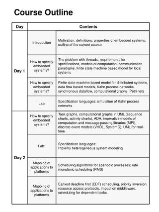
Course Outline. Traditional Static Program Analysis Theory Today: Compiler Optimizations, Control Flow Graphs Data-flow Analysis Classic analyses and applications Software Testing Dynamic Program Analysis. Textbooks.

Course Outline
E N D
Presentation Transcript
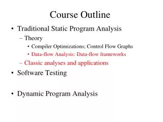
Course Outline • Traditional Static Program Analysis • Theory • Today: Compiler Optimizations, Control Flow Graphs • Data-flow Analysis • Classic analyses and applications • Software Testing • Dynamic Program Analysis
Textbooks • Compilers: Principles, Techniques and Tools by Aho, Lam, Sethi and UllmanAddison-Wesley 2007 • Principles of Program Analysis by Nielsen, Nielsen and Hankin, Springer 1999 • Notes, handouts and papers
Static Program Analysis • Analyzes the source code of the program and reasons about the run-time program behavior • Many uses • Traditionally in compilers in order to perform optimizing, semantics-preserving transformations • Recently in software tools for testing and validation: our focus
Outline • An Example: basic compiler optimizations • Control flow graphs • Local optimizations --- within basic blocks • Global optimizations --- across basic blocks • Reading: Compilers: Principles, Techniques and Tools, by Aho, Lam, Sethi and Ullman, Chapter 9.1
Compilation code optimizer code generator source program intermediate code intermediate code target program front end symbol table An optimization is a semantics-preserving transformation
Example • Define classical optimizations using an example Fortran loop • Opportunities result from table-driven code generation … sum = 0 do 10 i = 1, n 10 sum = sum + a[i]*a[i] …
Three Address Code • sum = 0 initialize sum • i = 1 initialize loop counter • if i > n goto 15 loop test, check for limit • t1 = addr(a) – 4 • t2 = i * 4 a[i] • t3 = t1[t2] • t4 = addr(a) – 4 • t5 = i * 4 a[i] • t6 = t4[t5] • t7 = t3 * t6 a[i]*a[i] • t8 = sum + t7 • sum = t8 increment sum • i = i + 1 increment loop counter • goto 3 • …
Control Flow Graph (CFG) • sum = 0 • i = 1 • if i > n goto 15 • t1 = addr(a) – 4 • t2 = i*4 • t3 = t1[t2] • t4 = addr(a) – 4 • t5 = i*4 • t6 = t4[t5] • t7 = t3*t6 • t8 = sum + t7 • sum = t8 • i = i + 1 • goto 3 T 15. … F
Common Subexpression Elimination • sum = 0 1. sum = 0 • i = 1 2. i = 1 • if i > n goto 15 3. if i > n goto 15 • t1 = addr(a) – 4 4. t1 = addr(a) – 4 • t2 = i*4 5. t2 = i*4 • t3 = t1[t2] 6. t3 = t1[t2] • t4 = addr(a) – 4 7. t4 = addr(a) – 4 • t5 = i*4 8. t5 = i*4 • t6 = t4[t5] 9. t6 = t4[t5] • t7 = t3*t6 10. t7 = t3*t6 • t8 = sum + t7 10a t7 = t3*t3 • sum = t8 11. t8 = sum + t7 • i = i + 1 11a sum = sum + t7 • goto 3 12. sum = t8 • … 13. i = i + 1 14. goto 3
Invariant Code Motion 1. sum = 0 1. sum = 0 2. i = 1 2. i = 1 • if i > n goto 15 2a t1 = addr(a) - 4 • t1 = addr(a) – 4 3. if i > n goto 15 5. t2 = i * 4 4. t1 = addr(a) - 4 • t3 = t1[t2] 5. t2 = i * 4 10a t7 = t3 * t3 6. t3 = t1[t2] 11a sum = sum + t7 10a t7 = t3 * t3 13. i = i + 1 11a sum = sum + t7 14. goto 3 13. i = i + 1 15. … 14. goto 3 15. …
Strength Reduction 1. sum = 0 1. sum = 0 2. i = 1 2. i = 1 2a t1 = addr(a) – 4 2a t1 = addr(a) - 4 3. if i > n goto 15 2b t2 = i * 4 5. t2 = i * 4 3. if i > n goto 15 6. t3 = t1[t2] 5. t2 = i * 4 10a t7 = t3 * t3 6. t3 = t1[t2] 11a sum = sum + t7 10a t7 = t3 * t3 13. i = i + 1 11a sum = sum + t7 14. goto 3 11b t2 = t2 + 4 15. … 13. i = i + 1 14. goto 3 15. …
Test Elision and Induction Variable Elimination 1. sum = 0 1. sum = 0 2. i = 1 2. i = 1 2a t1 = addr(a) – 4 2a t1 = addr(a) – 4 2b t2 = i * 4 2b t2 = i * 4 3. if i > n goto 15 2c t9 = n * 4 6. t3 = t1[t2] 3. if i > n goto 15 10a t7 = t3 * t3 3a if t2 > t9 goto 15 11a sum = sum + t7 6. t3 = t1[t2] 11b t2 = t2 + 4 10a t7 = t3 * t3 13. i = i + 1 11a sum = sum + t7 14. goto 3 11b t2 = t2 + 4 15. … 13. i = i + 1 14. goto 3a 15. …
Constant Propagation and Dead Code Elimination 1. sum = 0 1. sum = 0 2. i = 1 2. i = 1 2a t1 = addr(a) – 4 2a t1 = addr(a) - 4 2b t2 = i * 4 2b t2 = i * 4 2c t9 = n * 4 2c t9 = n * 4 3a if t2 > t9 goto 15 2d t2 = 4 6. t3 = t1[t2] 3a if t2 > t9 goto 15 10a t7 = t3 * t3 6. t3 = t1[t2] 11a sum = sum + t7 10a t7 = t3 * t3 11b t2 = t2 + 4 11a sum = sum + t7 14. goto 3a 11b t2 = t2 + 4 15. … 14. goto 3a 15. …
New Control Flow Graph 1. sum = 0 2. t1 = addr(a) - 4 3. t9 = n * 4 4. t2 = 4 5. if t2 > t9 goto 11 6. t3 = t1[t2] 7. t7 = t3 * t3 8. sum = sum + t7 9. t2 = t2 + 4 10. goto 5 T 11. … F
Building Control Flow Graph • Partition into basic blocks • Determine the leader statements (i) First program statement (ii) Targets of conditional or unconditional goto’s (iii) Any statement following a goto • For each leader, its basic block consists of the leader and all statements up to but not including the next leader or the end of the program
Building Control Flow Graph • Add flow-of-control information • There is a directed edge from basic block B1 to block B2 if B2 can immediately follow B1 in some execution sequence • B2 immediately follows B1 and B1 does not end in an unconditional jump • There is a jump from the last statement in B1 to the first statement in B2
Leader Statements and Basic Blocks • sum = 0 • i = 1 • if i > n goto 15 • t1 = addr(a) – 4 • t2 = i*4 • t3 = t1[t2] • t4 = addr(a) – 4 • t5 = i*4 • t6 = t5[t5] • t7 = t3*t6 • t8 = sum + t7 • sum = t8 • i = i + 1 • goto 3 • …
Analysis and optimizing transformations • Local optimizations – performed by local analysis of a basic block • Global optimizations – requires analysis of statements outside a basic block • Local optimizations are performed first, followed by global optimizations
Local optimizations --- optimizing transformations of a basic blocks • Local common subexpression elimination • Dead code elimination • Copy propagation • Constant propagation • Renaming of compiler-generated temporaries to share storage
Example 1: Local Common Subexpression Elimination • t1 = 4 * i • t2 = a [ t1 ] • t3 = 4 * i • t4 = b [ t3 ] • t5 = t2 * t4 • t6 = prod * t5 • prod = t6 • t7 = i + 1 • i = t7 • if i <= 20 goto 1
Example 2: Local Dead Code Elimination • a = y + 2 1’. a = y + 2 • z = x + w 2’. x = a • x = y + 2 3’. z = b + c • z = b + c 4’. b = a • b = y + 2
Example 3: Local Constant Propagation • t1 = 1 Assuming a, k, t3, and t4 are used beyond: • a = t1 1’. a = 1 • t2 = 1 + a 2’. k = 2 • k = t2 3’. t4 = 8.2 • t3 = cvttoreal(k) 4’. t3 = 8.2 • t4 = 6.2 + t3 • t3 = t4 • D. Gries’ algorithm: • Process 3-address statements in order • Check if operand is constant; if so, substitute • If all operands are constant, • Do operation, and add value to table associated with LHS • If not all operands constant Delete any table entry for LHS
Problems • Troubles with arrays and pointers. Consider: x = a[k]; a[j] = y; z = a[k]; Can we transform this code into the following? x = a[k]; a[j] = y; z = x;
Global optimizations --- require analysis outside of basic blocks • Global common subexpression elimination • Dead code elimination • Constant propagation • Loop optimizations • Loop invariant code motion • Strength reduction • Induction variable elimination
Global optimizations --- depend on data-flow analysis • Data-flow analysis refers to a body of techniques that derive information about the flow of data along program execution paths • For example, in order to perform global subexpression elimination we need to determine that 2 textually identical expressions evaluate to the same result along any possible execution path
Introduction to Data-flow Analysis • Collects information about the flow of data along execution paths • E.g., at some point we needed to know where a variable was last defined • Data-flow information • Data-flow analysis
1 2 3 4 5 6 7 8 9 10 Data-flow Analysis • G = (N, E, ρ) • Data-flow equations (also referred as transfer functions): • out(i) = gen(i) (in(i) – kill(i)) • Equations can be defined over basic blocks or over single statements. We will use equations over single statements
Four Classical Data-flow Problems • Reaching definitions (Reach) • Live uses of variables (Live) • Available expressions (Avail) • Very Busy Expressions (VeryB) • Def-use chains built from Reach, and the dual Use-def chains, built from Live, play role in many optimizations • Avail enables global common subexpression elimination • VeryB is used for conservative code motion
k n Reaching Definitions • DefinitionA statement that may change the value of a variable (e.g., x = i+5) • A definition of a variable x at node k reaches node n if there is a path clear of a definition of x from k to n. x = … x = … … = x
k n Live Uses of Variables • UseAppearance of a variable as an operand of a 3-address statement (e.g., y=x+4) • A use of a variable x at node n is live on exit from k if there is a path from k to n clear of definition of x. x = … x = … … = x
k n Def-use Relations • Use-def chain links an use to a definition that reaches that use • Def-use chain links a definition to an use that it reaches x = … x = … … = x
Optimizations Enabled • Dead code elimination (Def-use) • Code motion (Use-def) • Constant propagation (Use-def) • Strength reduction (Use-def) • Test elision (Use-def) • Copy propagation (Def-use)
Dead Code Elimination 1. sum = 02. i = 1 T 3. if i > n goto 15 F 4. t1 = addr(a)–45. t2 = i * 46. i = i + 1 After strength reduction, test elision and constant propagation, the def-use links from i=1 disappear. It becomes dead code.
Constant Propagation 1. i = 1 2. i = 1 3. i = 2 4. p = i*25. i = 1 6. q = 5*i+3 = 8
Terms • Control flow graph (CFG) • Basic block • Local optimization • Global optimization • Data-flow analysis