Course Outline
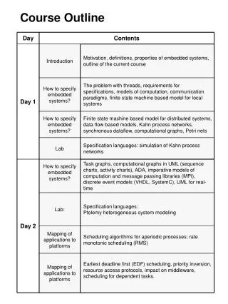
Course Outline. Traditional Static Program Analysis Theory Compiler Optimizations; Control Flow Graphs Data-flow Analysis: Data-flow frameworks Classic analyses and applications Software Testing Dynamic Program Analysis. Announcements. Homework 1 I will be done grading on Thursday


Course Outline
E N D
Presentation Transcript
Course Outline • Traditional Static Program Analysis • Theory • Compiler Optimizations; Control Flow Graphs • Data-flow Analysis: Data-flow frameworks • Classic analyses and applications • Software Testing • Dynamic Program Analysis
Announcements • Homework 1 • I will be done grading on Thursday • Homework 2 • Due Thursday, March 3rd • Problems with CS system • My other email: milana2@rpi.edu
Outline • Data-flow frameworks • Monotone frameworks • Distributive frameworks • The “Maximal Fixed Point” (MFP) solution • The “Meet Over all Paths” (MOP) solution • Analysis safety (correctness) and analysis precision • Reading: Compilers: Principles, Techniques and Tools, by Aho, Lam, Sethi and Ullman, Chapter 9.3
Monotone Dataflow Frameworks • Generic data-flow equations: in(i) = Vout(m)out(i) = fi(in(i)) Parameters: • Property space: in(i), out(i) are elements of a property space • Combination operator V:U for may problems and ∩for must problems • Initial values set to the 0 (smallest element) of the property space • Transfer functions: fiis associated with node i • If we instantiate these parameters in a certain way, then our analysis is an instance of the monotone dataflow framework m in pred(i)
Monotone Frameworks: Requirements • The property spacemust be a complete lattice L under partial order ≤where L satisfies the Ascending Chain Condition • The combination operator V • Initial values set to the 0 of L • The transfer functions: fi: L L Each fi must be monotone If fiis distributive,then our analysis is said to be distributive, a very special instance of the monotone dataflow framework
/* Initialize to initial values */ in(1)=InitialValue; in(1) = UNDEF for m := 2 to n do in(m) := 0; in(m) := Ø W := {1,2,…,n} /* put every node on the worklist */ while W ≠ Ø do { remove i from W; out(i) = fi(in(i)); outRD(i) = inRD(i)∩pres(i)Ugen(i) for j in successors(i) if out(i) ≤ in(j) then { if outRD(i) not subset of inRD (j) in(j) = out(i) V in(j); inRD(j) = out(i) U inRD(j) if j not in W do add j to W } } The Maximal Fixed Point (MFP)1 1. The Least Fixed Point (LFP) actually…
Properties of the algorithm • Lemma1: The algorithm terminates. Sketch of the proof: We have ink(j) ≤ ink+1(j) and since L has ACC, in(j) changes at most O(h) times. Each j is put on W at most O(h) times (h is the height of the lattice L). Complexity: At each iteration, the analysis examines e(j)out edges. Thus, number of basic operations is bounded by h*(e(1)out+…+e(N)out)=O(h*E). We can do better on certain graphs.
Properties of the Algorithm • Lemma2: The algorithm computes the least solution of the dataflow equations. • For every node i MFP computes solution MFP(i) = {in(i),out(i)}, such that every other solution {in’(i),out’(i)} of the dataflow equations is “larger” than the MFP • Lemma3: The algorithm computes a correct (safe) solution.
Example Solution1 Solution2 Ø Ø inAE(1) = Ø 1. z:=x+y {x+y} outAE(1)= (inAE(1)-Ez) {x+y} {x+y} inAE(2) = outAE(1)V outAE(3) {x+y} Ø 2. if (z > 500) outAE(2)= inAE(2) {x+y} Ø {x+y} Ø 3. skip inout(3) = outAE(2) {x+y} Ø outAE(3)= inAE(3) Equivalent to: inAE(2) = {x+y} V inAE(2) and recall that Vis ∩ (i.e., set intersection). That is why we needed to initialize inAE(2) and the other initial values to the universal set of expressions (0 of the Available Expressions lattice), rather than to the more intuitive empty set.
Meet Over All Paths (MOP) Solution1 ρ n1 n2 • Desired dataflow information at n is obtained by traversing ALL PATHS from ρ to n. For every path p=(ρ, n1, n2 ..., nk) we computefnk(…fn2(fn1(init(ρ)))) • The MOP at entry of n is Vfnk(…fn2(fn1(init(ρ)))) • The MOP is the best summary of dataflow facts possible to compute with this static analysis … nk n p in paths from ρto n
MOP vs. MFP • For distributive functions the dataflow analysis can merge paths (p1, p2), without loss of precision! • E.g., fp1(0) need not be calculated explicitly • MFP=MOP • Due to Kam and Ullman, 1976,1977: This is not true for monotone functions. • Lemma 3: The MFP approximates the MOP for general monotone functions: MFP ≥ MOP
Safety of a Dataflow Solution • Safe (also, correct or sound) solution overestimates the best possible dataflow solution, i.e., x ≥ MOP is an approximate solution • Acceptable solution is better than what we can do with the MFP, i.e., x ≤ MFP • Between MOP and MFP are interesting solutions MFP Acceptable Safe MOP 0
Precision of a Dataflow Solution • Precise solution is one that is close to MOP • A precise solution contains few spurious facts • MOP ≤ X ≤ Y: X is more precise than Y
Safe Solutions • In Available Expressions the 1 is the empty set, and the combination operator is set intersection. • It is safe to err by saying that an expression is NOT AVAILABLE when it might be. • We compute a smaller set. Thus, under our definition of ≤, this solution is larger than the MOP. • In Reaching Definitions the 1 is the universal set of definitions, the combination is the union. • It is safe to err by saying that a definition reaches a node when in fact it DOES NOT REACH the node. • We compute a larger set. Thus, under our definition of ≤ (which is natural), the solution is larger than the MOP
Two Views of Reaching Definitions Defs Safe solutions are here; they are larger sets of definitions. MOP/MFP 0 element Join semi-lattice formulation. We used this formulation.
Two Views of Reaching Definitions Ø 1 element def1 … defk . . MOP/MFP Safe solutions are larger sets of definitions than MOP Defs Meet semi-lattice formulation
Kam and Ullman Results • On monotone dataflow frameworks, iterative algorithms converge to the MFP of the dataflow equations (our Lemmas 1 and 2) • MOP ≤ MFP (in our join formulation) (our Lemma 3) • One monotone framework that is not distributive is constant propagation • The MOP is undecidable for an arbitrary instance of a monotone framework.
Many Applications! • White-box testing: compute coverage • Control-flow-based testing • Data-flow-based testing • Intuitively, test each def-use chain • Regression testing • Analyze changes and select regression tests that actually test changed code
Many Applications! • Reverse engineering • UML class diagrams • UML sequence diagrams • Many tools do these; Eclipse plug-ins • Automated refactoring • Analyze program, prove “safety” of the refactoring • Eclipse plug-ins
Many Applications! • Static debugging • Memory errors in C/C++ programs • Memory leaks • Null pointer dereferences • Array-out-of-bound accesses • Concurrency errors in shared-memory apps • Data-races • Atomicity violations • Deadlocks