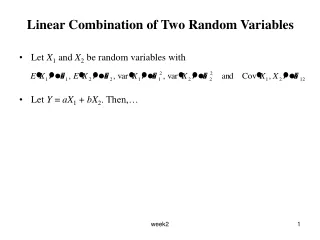
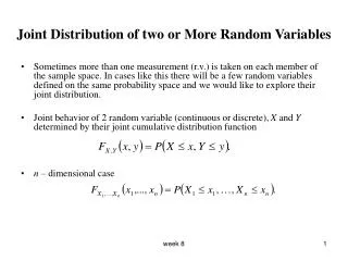
Joint Distribution of two or More Random Variables

1. Joint Distribution of two or More Random Variables • Sometimes more than one measurement (r.v.) is taken on each member of the sample space. In cases like this there will be a few random variables defined on the same probability space and we would like to explore their joint distribution. • Joint behavior of 2 random variable (continuous or discrete), X and Y determined by their joint cumulative distribution function • n – dimensional case week 8

2. Discrete case • Suppose X, Y are discrete random variables defined on the same probability space. • The joint probability mass function of 2 discrete random variables X and Y is the function pX,Y(x,y) defined for all pairs of real numbers x and y by • For a joint pmf pX,Y(x,y) we must have: pX,Y(x,y) ≥ 0 for all values of x,y and week 8

3. Example for illustration • Toss a coin 3 times. Define, X: number of heads on 1st toss, Y: total number of heads. • The sample space is Ω ={TTT, TTH, THT, HTT, THH, HTH, HHT, HHH}. • We display the joint distribution of X and Y in the following table • Can we recover the probability mass function for X and Y from the joint table? • To find the probability mass function of X we sum the appropriate rows of the table of the joint probability function. • Similarly, to find the mass function for Y we sum the appropriate columns. week 8

4. Marginal Probability Function • The marginal probability mass function for X is • The marginal probability mass function for Y is • Case of several discrete random variables is analogous. • If X1,…,Xm are discrete random variables on the same sample space with joint probability function The marginal probability function for X1 is • The 2-dimentional marginal probability function for X1 and X2 is week 8

5. Example • Roll a die twice. Let X: number of 1’s and Y: total of the 2 die. There is no available form of the joint mass function for X, Y. We display the joint distribution of X and Y with the following table. • The marginal probability mass function of X and Y are • Find P(X ≤ 1 and Y≤ 4) week 8

6. Independence of random variables • Recall the definition of random variable X: mapping from Ω to R such that for . • By definition of F, this implies that (X > 1.4) is and event and for the discrete case (X = 2) is an event. • In general is an event for any set A that is formed by taking unions / complements / intersections of intervals from R. • Definition Random variables X and Y are independent if the events and are independent. week 8

7. Theorem • Two discrete random variables X and Y with joint pmf pX,Y(x,y) and marginal mass function pX(x) and pY(y), are independent if and only if • Proof: • Question: Back to the rolling die 2 times example, are X and Y independent? week 8

8. Conditional Probability on a joint discrete distribution • Given the joint pmf of X and Y, we want to find and • Back to the example on slide 5, • These 11 probabilities give the conditional pmf of Y given X = 1. week 8

9. Definition • For X, Y discrete random variables with joint pmf pX,Y(x,y) and marginal mass function pX(x) and pY(y). If x is a number such that pX(x) > 0, then the conditional pmf of Y given X = x is • Is this a valid pmf? • Similarly, the conditional pmf of X given Y = y is • Note, from the above conditional pmf we get Summing both sides over all possible values of Y we get This is an extremely useful application of the law of total probability. • Note: If X, Y are independent random variables then PX|Y(x|y) = PX(x). week 8

10. Example • Suppose we roll a fair die; whatever number comes up we toss a coin that many times. What is the distribution of the number of heads? Let X = number of heads, Y = number on die. We know that Want to find pX(x). • The conditional probability function of X given Y = y is given by for x = 0, 1, …, y. • By the Law of Total Probability we have Possible values of x: 0,1,2,…,6. week 8

11. Example • Interested in the 1st and 2nd success in repeated Bernoulli trails with probability of success p on any trail. Let X = number of failures before 1st success and Y = number of failures before 2nd success (including those before the 1st success). • The marginal pmf of X and Y are for x = 0, 1, 2, …. • and for y = 0, 1, 2, …. • The joint mass function, pX,Y(x,y) , where x, y are non-negative integers and x ≤ y is the probability that the 1st success occurred after x failure and the 2nd success after y – x more failures (after 1st success), e.g. • The joint pmf is then given by • Find the marginal probability functions of X, Y. Are X, Y independent? • What is the conditional probability function of X given Y = 5 week 8

12. Some Notes on Multiple Integration • Recall: simple integral cab be regarded as the limit as N  ∞ of the Riemann sum of the form where ∆xi is the length of the ith subinterval of some partition of [a, b]. • By analogy, a double integral where D is a finite region in the xy-plane, can be regarded as the limit as N  ∞ of the Riemann sum of the form where Ai is the area of the ith rectangle in a decomposition of D into rectangles. week 8

13. Evaluation of Double Integrals • Idea – evaluate as an iterated integral. Restrict D now to a region such that any vertical line cuts its boundary in 2 points. So we can describe D by yL(x) ≤ y ≤ yU(x) and xL ≤ x ≤ xU • Theorem Let D be the subset of R2 defined by yL(x) ≤ y ≤ yU(x) and xL ≤ x ≤ xU If f(x,y) is continuous on D then • Comment: When evaluating a double integral, the shape of the region or the form of f (x,y) may dictate that you interchange the role of x and y and integrate first w.r.t x and then y. week 8

14. Examples 1) Evaluate where D is the triangle with vertices (0,0), (2,0) and (0,1). 2) Evaluate where D is the region in the 1st quadrate bounded by y = 0, y = x and x2 + y2 = 1. 3) Integrate over the set of points in the positive quadrate for which y > 2x. week 8

15. The Joint Distribution of two Continuous R.V’s • Definition Random variables X and Y are (jointly) continuous if there is a non-negative function fX,Y(x,y) such that for any “reasonable” 2-dimensional set A. • fX,Y(x,y) is called a joint density function for (X, Y). • In particular , if A = {(X, Y): X ≤ x, Y ≤ x}, the joint CDF of X,Y is • From Fundamental Theorem of Calculus we have week 8

16. Properties of joint density function • for all • It’s integral over R2 is week 8

17. Example • Consider the following bivariate density function • Check if it’s a valid density function. • Compute P(X > Y). week 8

18. Properties of Joint Distribution Function For random variables X, Y , FX,Y : R2 [0,1] given by FX,Y (x,y) = P(X ≤ x,Y ≤ x) • FX,Y (x,y) is non-decreasing in each variable i.e. if x1 ≤x2 and y1 ≤y2 . • and week 8

19. Marginal Densities and Distribution Functions • The marginal (cumulative) distribution function of X is • The marginal density of X is then • Similarly the marginal density of Y is week 8

20. Example • Consider the following bivariate density function • Check if it is a valid density function. • Find the joint CDF of (X, Y) and compute P(X ≤ ½ ,Y≤ ½ ). • Compute P(X ≤ 2 ,Y≤ ½ ). • Find the marginal densities of X and Y. week 8

21. Generalization to higher dimensions Suppose X, Y, Z are jointly continuous random variables with density f(x,y,z), then • Marginal density of X is given by: • Marginal density of X, Y is given by: week 8

22. Example Given the following joint CDF of X, Y • Find the joint density of X, Y. • Find the marginal densities of X and Y and identify them. week 8

23. Example Consider the joint density where λ is a positive parameter. • Check if it is a valid density. • Find the marginal densities of X and Y and identify them. week 8