Download
1 / 36
360 likes | 380 Vues
Explore interactions of solar wind with unmagnetized bodies like moons and asteroids in space. Learn about plasma flow absorption, wakes formation, and induced electrical currents. Discover how weakly-atmosphered bodies interact with solar wind.

E N D
ESS154/200C Lecture 10Solar Wind Interactions: Unmagnetized Planets
ESS 200C Space Plasma Physics ESS 154 Solar Terrestrial PhysicsM/W/F 10:00 – 11:15 AM Geology 4677 Instructors:C.T. Russell (Tel. x-53188; Office: Slichter 6869)R.J. Strangeway (Tel. x-66247; Office: Slichter 6869) • DateDayTopicInstructorDue • 1/4 M A Brief History of Solar Terrestrial Physics CTR • 1/6 W Upper Atmosphere / Ionosphere CTR • 1/8 F The Sun: Core to Chromosphere CTR • 1/11 M The Corona, Solar Cycle, Solar Activity Coronal Mass Ejections, and Flares CTR PS1 • 1/13 W The Solar Wind and Heliosphere, Part 1 CTR • 1/15 F The Solar Wind and Heliosphere, Part 2 CTR • 1/20 W Physics of Plasmas RJS PS2 • 1/22 F MHD including Waves RJS • 1/25 M Solar Wind Interactions: Magnetized Planets YM PS3 • 1/27 W Solar Wind Interactions: UnmagnetizedPlanets YM • 1/29 F CollisionlessShocks CTR • 2/1 M Mid-Term PS4 • 2/3 W Solar Wind Magnetosphere Coupling I CTR • 2/5 F Solar Wind Magnetosphere Coupling II; The Inner Magnetosphere I CTR • 2/8M The Inner Magnetosphere II CTR PS5 • 2/10W Planetary Magnetospheres CTR • 2/12F The Auroral Ionosphere RJS • 2/17W Waves in Plasmas 1 RJS PS6 • 2/19 F Waves in Plasmas 2 RJS • 2/26 F Review CTR/RJS PS7 • 2/29 M Final
Interactions with Atmosphereless Bodies • If a body in a flowing magnetized space plasma is nonconducting or only partially conducting, like rock or ice, some or all of the incident flow is absorbed on the plasma ram face. • The absorbed plasma leaves a wake behind the moon. If the magnetic field is parallel to the flow, the wake does not close (fill in) completely farther downstream. If the magnetic field is perpendicular to the floe, the wake closes along the field at the thermal speed. The field in the wake is only modestly distorted from the undisturbed external field in both cases. • The external flows may be solar wind or magnetospheric, and the bodies involved may be planetary satellites or asteroids. Examples of such interactions include the Earth’s moon, Tethys, Rhea, Dione at Saturn. Note that sputtering of the surface by the incident particles may also form a rudimentary atmosphere, usually an exosphere, on the plasma ram face, but we ignore this here.
Interactions with Atmosphereless Bodies • When the body has a low conductivity surface layer but an interior ‘core’ of both significant size and conductivity, the electrical currents induced in that conductor can persist sufficiently long to exclude the magnetic field from the conducting region. • If the conducting region is large compared to the size of the body then a very large disturbance can be produced (above left), and sometimes detected. • This effect can be used to sound the size of the core and has been used on our Moon. It can be measured when the Moon enters the lobes of the Earth magnetotail where external fields are quiet and only slowly varying.
Interactions with Bodies with Weak Atmospheres • Bodies with weak atmospheres or exospheres may lose mass to the solar wind flow via photo-ionization or impact ionization or charge exchange followed by the ion pick-up via the Lorentz force. As described in the solar wind lecture, the pickup ion drifts at the plasma flow speed in a cycloid perpendicular to the magnetic field if the plasma flow and field are perpendicular. • The momentum required for the pick-up particles is extracted from the ambient flow, whether solar wind or magnetospheric. This is often referred to as ‘mass loading’ of the plasma because the newly produced ions usually add mass to the original flow (the exception is for a few special cases such as H+ charge exchange with H). • Since gyro-radii are mass-dependent, a mass spectrometer effect occurs in which some ions with small gyroradii compared to the body size may impact it while others manage to avoid impact. The latter can escape if their speeds exceed the escape velocity for the body, determined by its gravity and size. The impact of these atmospheric ions can cause additional sputtering loss. Bottom: illustration of pickup Ion impact on Earth’s Moon from Manka and Michel, 1973
Interactions with Bodies with Thick Atmospheres and No Magnetic field • When a body has a substantial atmosphere, and is sufficiently close to the Sun, solar EUV photons partially ionize the dayside to produce an ionosphere. • When the external plasma flow arrives, it could impact the atmosphere and be absorbed if there is no magnetic field. But if the incident plasma is magnetized, currents are induced in the conducting ionosphere that oppose the external magnetic field and counter its penetration (diamagnetic currents). • Eventually (months?) these currents would decay, but if the direction of the field keeps changing, the field is excluded. What is happening is δB/δt induction. These ionospheric currents form a magnetic barrier that can exclude the external magnetic field from the ionosphere and lead to a magnetosheath-like structure with draped interplanetary fields. This type of interaction is often referred to as an ‘induced magnetosphere’. Venus is our best example of this.
The Ionospheric Obstacle: Ionopause The ionosphere is the obstacle to the solar wind. The boundary between the ionosphere and the shocked and slowed solar wind is called the ionopause. Around solar maximum, the ionopause is located at about 400 km altitude at the subsolar point and around 1000 km at the terminator. The ionosphere thickness is quite small compared to the planet radius, and so the obstacle is almost planet-sized and much smaller than the magnetosphere of Earth (Venus’ twin in planet size). 7
Size of the Ionospheric Obstacle • The solar wind flow exerts dynamic pressure plus magnetic and thermal pressure. The ionosphere exerts mainly thermal pressure force against the solar wind. Along the stagnation line of the interaction, approximate pressure balance is achieved. • As the incident solar wind changes, or the ionosphere thermal pressure changes (e.g. due to solar EUV variations) the ionosphere moves. It goes to lower altitudes as the external pressure increases but has a limit at around the exobase altitude (at Venus ~200km). Below this altitude the ionosphere is photochemically controlled, meaning production rather than dynamics dictates the thermal pressure. • If the thermal pressure at the peak of the ionosphere is greater than the dynamic pressure of the incident flow, and the standoff distance is well above the collisional region of the atmosphere (e.g. above the exobase), then the magnetic field is largely excluded from the ionosphere. If the peak ionospheric thermal pressure is lower than the external plasma pressure, the magnetic field collisonally diffuses into the ionosphere to contribute to its pressure and reinforce its obstacle-like effects on the oncoming flow. Such ‘magnetized ionospheres’ were first seen at Venus. 8
The Bow Shock Location • The Venus Bow Shock position is observed to change in response to solar EUV flux (Left figures). It is also expected that the ionosphere is generally more magnetized but we lack observations of the solar minimum subsolar ionosphere. • The general idea of how the Venus interaction changes from solar maximum to minimum in the form of the draped magnetic field geometry, is suggested in the right-hand sketch above. However Venus Express observations around solar minimum indicate the actual geometry may involve both configurations, depending on the hemisphere relative to the convection electric field direction.
The Magnetic Barrier External solar wind pressure nswkTsw + ρv2 + B2 / 2μ0 Is mainly dynamic Dynamic pressure goes to Magnetic pressure goes to Ionospheric thermal Pressure (magnetic contributions can remain) Along the stagnation line pressure balance occurs and a transition is observed from solar wind dynamic pressure to magnetic pressure in the inner draped field/magnetosheath region, to the ionosphere where thermal plasma pressure dominates. The layer where the draped magnetic field pileup takes most of the pressure has been referred to as a ‘magnetic barrier’ or pileup region (from Russell and Vaisberg in VENUS, Univ of Arizona Press, 1982)
Flux Ropes in Planetary Ionospheres • The large scale fields are absent when the ionopause is high (~ 300 km subsolar), or decay if they were present. In some cases, typical for solar maximum, bundles of magnetic flux resembling flux ropes are observed in the dayside ionosphere. These fields (e.g. from weak downward diffusion or decayed fields) become force-free so that the twist in the field balances the magnetic pressure gradient. • In a force-free rope, the current is parallel to the magnetic field. If j = αB andαis constant, this is called a Taylor state, and the field components (axial and azimuthal) are described by Bessel functions. • The bottom panel above right illustrates the distribution of flux ropes in the Venus ionosphere, viewed in cross section. In this sketch the barrier and axial fields point out of the page. However some analyses suggest they are often twisted and kinked.
The Magnetosheath The magnetosheath fields at Venus fit models remarkably well (here a gas-dynamic field model was used). The ionosphere acts like a conducting sphere in this case.
Numerical Simulations of Venus 1 MHD simulations can replicate many average properties of the Venus-solar wind interaction. The solar wind hydrogen plasma and the ionospheric plasma are the main ‘fluids’ represented. The simulations use an atmosphere Model (Venus has a mostly CO2 and O atmosphere) with ions produced by ‘exposing’ the atmosphere to solar EUV (photo-ionization), impact ionization by solar wind electrons, and charge exchange with solar wind protons. The model results show the magnetic field strength (contour) and directions (white arrows) (left panels) and flow speed and directions (right panels) (right panels). As in the real case, an induced magnetospheric obstacle is produced. Sample of PVO magnetic field strength averages folded into a plane. Dark blue areas are not sampled. Here the Sun is at left. 13
This figure shows both the upstream and downstream views of the interaction process. The gray isosurface represents a density contour with planetary O+ density equals to 50/cc as an indication of Venus ionosphere, which is around 400 km altitude along the subsolar line, but extends nearly to 5 RV in the nightside. This figure shows how field lines wrap around the obstacle on the upstream side, but slip over the obstacle on the night side. The field lines at high latitude are kinked because the plasma closer to the planet have been mass-loaded by planetary ion production and so significantly slowed down as compared with plasma further away from the planet. The draped field exerts a JxB force on the plasma in the wake, speeding it up to escape velocity as down-tail distance increases. 14
The MHD simulations of the Venus solar wind interaction can be used to study the ion escape associated with thermal pressure gradient , convection electric field –VxB, and JxB forces. Here the loss of O+ in the wake is illustrated by color contours of the ion density in the equatorial plane views for solar max and min cases. (The interplanetary field orientation is equatorial) The escape velocity for Venus is ~11 km/s so all ions moving tailward above this speed are permanently lost to the planet. The rates are ~3-5X1025 s-1. Such escape processes acting over time can affect the planet’s atmosphere evolution. 15
Atmospheric Erosion 1- Superthermal Atoms • The Venus exosphere has a hot hydrogen and a hot oxygen component. The hot oxygen is produced by the dissociative recombination of the primary ion O2+ e + O2+ → O* + O* (here * indicates a neutral O atom with supra-thermal energy from the process) • Some of these suprathermal atoms are upward-directed and reach high altitudes. Like any thermal atoms above the ionopause, these atoms can be ionized by photoionization, impact ionization and charge exchange and can add to the production of ions directly exposed to solar wind convection electric fields. These ions are then subject to the ion pickup process.
ion trajectory if Vsw=0 Convection E field=-Vsw x B accelerates the ion here B field Vsw Incident Plasma flow Pickup Ion trajectory Atmospheric Erosion 2-Loss due to ion pickup Recall how the ion pickup process works. One can think of it as ions becoming entrained on moving field lines. (Note in the lefthand picture, in a frame moving at Vsw the ion is simply gyrating around the field.) In this case the moving magnetic field is provided by the solar wind, and ions by the atmosphere and various ionization processes. Because the solar wind speed is high and even the shocked solar wind in the magnetosheath has fast flows (see MHD model velocities) the ions that are picked up can reach velocities above the ~11 km/s escape velocity.
Atmospheric Erosion-Observations and Models PVO Plasma Analyzer detections of inferred escaping O+ ions organized by the Interplanetary Magnetic Field (IMF) direction show the spatial asymmetryexpected for the ion pickup process, characterized by a preference for the –VxB electric field hemisphere.Test particle pickup ions showing the expected asymmetries for IMF in east and west orientations. These are based on magnetic fields and flows from an MHD model. Cross-flow IMF
An ionospheric obstacle with crustal fields The Mars-solar wind interaction represents an ionospheric interaction but with further complications compared to Venus: • There are significant crustal remnant magnetic fields present. • The gyroradius of the incident solar wind protons is more comparable to the scale of the interaction features (e.g. the subsolar magnetosheath), making microscopic or kinetic effects more important overall.
A few field lines traced in the Purucker model of the Mars crustal magnetic field (only). the surface is color coded by the radial field strength (Red and blue are strong +/- field). The strongest fields are in the southern hemisphere. Crustal field intrusions in MGS Magnetic field data and their apparent effects on the magnetosheath field draping show the need for more complicated models for Mars
The Ionosphere of Mars • The Mars and Venus ionospheres, illustrated by the photochemical models shown in the upper figure panels are similar but not identical. • Although both are mainly O2+ at the ionosphere peak, Venus has higher densities of atomic oxygen ions above the peak. • At both planets, the observed ion density at high altitudes is less than expected, consisted with erosion/escape at the top (bottom panels).
Mars’ Atmospheric Loss Mars is smaller than Venus and has lower surface gravity. While dissociative recombination-enabled escape of O (O2+ + e ->2O*) doesn’t work on Venus (need 10 eV (vesc=11 km/s O)), it dominates all other O escape processes for Mars (needs only 2 eV (vesc=5 km/s O)). Ionospheric ‘source’ From Shinagawa, JASR, 2005
Numerical Simulations for Mars Sophisticated numerical models are necessary to understand the complicated geometry of the Mars solar wind interaction and to interpret the phenomena observed in the plasma interaction. The figures show calculated magnetic field and velocity in the meridianal plane for a typical case. The color plots show the magnitudes; the white lines marked with arrows indicate the vector direction of the magnetic field and the arrows show the direction (not the magnitude) of the velocity. The dashed line represents the mean bow shock and the dash-dot line is the mean MPB locations from Vignes et al. [2000]
Ma et al. model ionosphere at various locations vs. Viking data SZA=45 SZA=0 SZA=45 This self-consistent MHD model with an ionosphere reproduces the Viking Lander profiles as well as the bow shock position.
Sub-Alfvenic, steady field interactions: Alfven Wings When the magnetic field is strong so that the flow is sub-Alfvenic, the field lines bend but do not strongly drape. If the flow across the polar cap becomes very slow perhaps due to intense mass loading, then the flux tube is essentially frozen to the moon (e.g. Io) and the other flux tubes have to move around the Alfven wing field lines rooted to the moon. The extensions of the penetrated flux tubes are called ‘Alfven wings’. They can be detected far from the body itself, at increasing distances from the wake axis. Jupiter’s satellite Io was the inspiration for work on this type of interaction although many magnetosphere-satellite interactions at the giant planets are likely of this type. 25
Alfven Wing plus Ionosphere Interactions Saturn’s large (~2275 km radius) satellite Titan has a thick atmosphere that makes it like a small planet. It typically resides in Saturn’s magnetosphere although at ~20 Rsaturn orbital distance it sometimes crosses the magnetopause into Saturn’s magnetosheath. The Cassini mission is exploring its plasma interaction.
Titan’s orbit (red) is near the Magnetopause and goes in and out of the bowl-like plasma disk Complications of the Titan interaction include a changing geometry between the sunlit face of Titan where the main ionosphere is produced, and the oncoming magnetospheric flow that corotates with Saturn. Also the local field is not so dipolar, and proximity to magnetopause and magnetotail make its environment variable.
Titan’s ionosphere Titan’s upper atmosphere is mainly molecular nitrogen and methane- whilethe ionosphere is a rich mix of hydrocarbon ions. Thus it does not have thesame photochemistry as Venus and Mars. (Cassini INMS profiles of atmospheric neutrals from Waite et al., Science, 2005) (modeled dayside ionosphere From Ma et al., JGR, 2007)
Single-Fluid MHD Model Results in the Ideal Case U U E0 B0 U B U-B Plane U-E Plane The top two panels show plasma flow speed(contour color) and direction (white arrows) in both U-E and U-B planes. The bottom two panels show magnetic field strength (contour color) and direction(white arrows) in both U-E and U-B planes. The single fluid MHD model results are symmetric in UE plane because in this model, the mass-loading effect is included but the gyroradii of the pick-up ions are neglected. 29
Multi-Fluid MHD Model Results in the Ideal Case U U E0 B0 U B U-E Plane U-B Plane The multi-fluid MHD model allows the motions of different ion fluids to be decoupled, and it was able to reproduce the asymmetric results along the convection electric field direction (similar to hybrid model results). Multi-fluid MHD model also predicts that more heavy ions are escaping from Titan. 30
SLT Effect– 18 SLT vs. 6 SLT u0 E0 Sun Sun The figures show the density distribution(contour) of two different mass fluids: mass 1(upper panels) and mass 28(lower panels) over plotted with the corresponding flow vector(the white arrows) in the UE plane. The plasma interaction also depends on Titan’s orbital location as shown in the two cases: 18 SLT(left panels) vs. 6 SLT(right panels). 31
Interactions including Plumes and Volcanoes • The interiors of some moons are outgassing rapidly with much of that gas escaping. • Io has volcanoes. • Enceladus has a southern polar plume from fissures that vent mainly water ice and dust. • Enceladus’ plume extends far south of it so the central mass-loading point is well below the moon. • MHD simulations with charge-exchange, impact and photoionization can mimic the variation in the magnitude of the perturbation but not the components, indicating that there are forces and flows we are not properly calculating. Enceladus’ Plume
The Cometary Interaction • When comets approach the Sun, they heat up and outgas. • The expanding gas decreases in density and is lost through photoionization where u is the outflow velocity (~km/s) and τ the photoionization time scale. • The comet can produce a small field-free region around the nucleus where cometary ions dominate , but the region of draped interplanetary magnetic field due to cometary ion pickup producing solar wind mass loading is huge.
Cometary Simulations • A numerical simulation of this process shows that the stream lines of the flow do not become very diverted but flow almost straight through the mass-loading region. Note the scales. • The field lines become draped and eventually straighten far downstream. • Comets also produce lots of dust. This dust is charged and can interact with the solar wind like very heavy pickup ions.
Space Weather Effects at Unmagnetized Bodies Periods of Venus obstacle Encounters Once/day Interplanetary magnetic field associated with an ICME Many ICMEs and SEP events are observed going past Venus (here an ICME seen on PVO) and Mars, but the of study their effects (e.g. on atmosphere escape) has yet to be carried out in depth. This is a project for the coming years.
Summary and Conclusions • The interaction of flowing magnetized plasmas with atmosphereless bodies can tell us about the surface and interior of the body. • If there is a weak atmosphere, it can be probed using the IMF to produce a mass spectrum. • A thick atmosphere can support an ionosphere which can be sufficiently electrically conducting that the interplanetary magnetic field is excluded from the ionosphere. This forms a magnetic barrier that deflects the solar wind and forms a shock. A magnetotail forms. There may be large scale fields or flux ropes in the ionosphere. • Some moons outgas rapidly in plumes and volcanoes and also form mass-loading obstacles. Charge-exchange producing fast neutrals is also important. • Comets are active outgassing bodies that mass load the solar wind. Although the smallest bodies, comets can produce some of the largest unmagnetized plasma interactions in the solar system.