SOLAR DYNAMO MODELING AND PREDICTION
290 likes | 540 Vues
SOLAR DYNAMO MODELING AND PREDICTION. Mausumi Dikpati High Altitude Observatory, NCAR. Observational signature for global evolution of solar magnetic fields. From url of D. Hathaway. What is a dynamo?. All these magnetic fields are maintained by dynamo action.

SOLAR DYNAMO MODELING AND PREDICTION
E N D
Presentation Transcript
SOLAR DYNAMO MODELING AND PREDICTION Mausumi DikpatiHigh Altitude Observatory, NCAR
Observational signature for global evolution of solar magnetic fields From url of D. Hathaway
What is a dynamo? All these magnetic fields are maintained by dynamo action A dynamo is a process by which the magnetic field in an electrically conducting fluid is maintained against Ohmic dissipation In astrophysical object, there can always be a dynamo whenever the plasma consists of seed magnetic fields and flow fields
Flux-transport Dynamo < (i) Generation of toroidal (azimuthal) field by shearing a pre-existing poloidal field (component in meridional plane) by differential rotation (Ω-effect ) (ii) Re-generation of poloidal field by lifting and twisting a toroidal flux tube by helical turbulence (α-effect) (iii) Flux transport by meridional circulation
Fixing dynamo ingredients While Ω -effect and meridional circulation can be fixed from observations, the α–effect could be of different types as suggested theoretically. One directly observed α–effect can arise from decay of tilted, bipolar active regions Babcock 1961, ApJ, 133, 572
How a Babcock-Leighton Flux-transport dynamo works Shearing of poloidal fields by differential rotation to produce new toroidal fields, followed by eruption of sunspots. Spot-decay and spreading to produce new surface global poloidal fields. Transport of poloidal fields by meridional circulation (conveyor belt) toward the pole and down to the bottom, followed by regeneration of new toroidal fields of opposite sign.
Mathematical Formulation Toroidal field Poloidal field Meridional circulation Differential rotation Under MHD approximation (i.e. electromagnetic variations are nonrelativistic), Maxwell’s equations + generalized Ohm’s law lead to induction equation : (1) Applying mean-field theory to (1), we obtain the dynamo equation as, (2) Turbulent magnetic diffusivity Differential rotation and meridional circulation from helioseismic data Poloidal field source from active region decay Assume axisymmetry, decompose into toroidal and poloidal components:
Poloidal and Toroidal Equations and Boundary Conditions (3a) (3b) (i) Both poloidal and toroidal fields are zero at bottom boundary (ii) Toroidal field is zero at poles, whereas poloidal field is parallel to polar axis (iii) Toroidal field zero at surface; poloidal fields from interior match potential field above surface (iv) Both poloidal and toroidal fields are antisymmetric about the equator
Evolution of Magnetic FieldsIn a Babcock-Leighton Flux-Transport Dynamo Dynamo cycle period ( T ) primarily governed by meridional flow speed Dikpati & Charbonneau 1999, ApJ, 518, 508
Refining a Babcock_Leighton flux-transport dynamo A full-spherical-shell Babcock-Leighton dynamo relaxes to a quadrupole parity, violating the observed Hale’s polarity rule which implies dipole parity about the equator Remedy: a tachocline α-effect Dikpati & Gilman, 2001, ApJ, 559, 428; Bonanno et al, 2002, A&A, 390, 673
Calibrated Flux-transport Dynamo Model Flows derived from observations Magnetic diffusivity used N-Pole Red: α -effect location Green: rotation contours Blue: meridional flow Near-surface diffusivity same as used by Wang, Shelley & Lean, 2002; Schrijver 2002 in their surface flux-transport models. Zita is exploring in details the sensitivity of diffusivity profiles to flux-transport dynamo S-Pole
Validity test of calibration Contours: toroidal fields at CZ base Gray-shades: surface radial fields Observed NSO map of longitude-averaged photospheric fields Dikpati, de Toma, Gilman, Arge & White, 2004, ApJ, 601, 1136
Why is solar cycle prediction important? • High atmosphere density varies as function of solar cycle • Density variation at 400 km depth is 2-3 times that of cycle amplitude variation • Satellites are placed at that altitude, and so drag due to density variation affects their lifetime Qian, Solomon & Roble; GRL, 2006
Issues with polar field precursor techniques < < < 3. Strong radial; weak latitudinal 2. Weak radial; weak latitudinal 1. Weak radial; strong latitudinal Q1. How can the 5.5 year-old polar fields from previous cycle determine the next cycle’s amplitude? Q2. Do they remain radial down to shear layer? Q3. Are stronger radial fields associated with stronger or weaker latitudinal fields? It depends on field geometry inside convection zone: see 3 possible cases
Flux-transport dynamo-based prediction scheme Meridional circulation plays an important role in this class of model, by governing a) the dynamo cycle period b) the memory of the Sun’s past magnetic fields <
Timing Prediction For Cycle 24 Onset Dikpati, 2004, ESA-SP, 559, 233
Recent Support For Delayed Onset Of Cycle 24 Cycle 23 onset Pred. cycle 24 onset
Recent Support For Delayed Minimum At End of Cycle 23 Mar. 29, 2006 Nov. 1994 Early 1996 This coronal structure not yet close to minimum; more like 18 months before minimum Corona at last solar minimum looked like this
Amplitude prediction: Data-assimilation In Solar Cycle Models • Given the strong correlation between area and flux, we apply data-assimilation techniques to our calibrated dynamo • Such techniques used in meteorology for 50 years, but just starting in solar physics • Appropriate time for data-assimilation in solar physics: large new data-sets becoming available • First example; predicting relative solar cycle peaks. • Future goal: simultaneous predictions of cycle amplitude and timing, using “sequential” and “variational” data-assimilation techniques
Construction Of Surface Poloidal Source: 2D Data Assimilation Original data (from Hathaway) Period adjusted to average cycle Assumed pattern extending beyond present
Three techniques for treating surface poloidal source in simulating and forecasting cycles Forecasted quantity : integrated toroidal magnetic flux at the bottom in latitude range of 0 to 45 degree (which is the sunspot-producing field) 1) Continuously update of observed surface source including cycle predicted (a form of 2D data assimilation) 2) Switch off observed surface source for cycle to be predicted 3) Substitute theoretical surface source, derived from dynamo-generated toroidal field at the bottom, for observed surface source We use these three techniques in succession to simulate and forecast
Simulating Relative Peaks Of Cycles 12 Through 24 • We reproduce the sequence of peaks of cycles 16 through 23 • We predict cycle 24 will be 30-50% bigger than cycle 23 Dikpati, de Toma & Gilman, 2006, GRL, 33, L05102
Evolution of predictive solution Toroidal field Latitudinal field Color shades denote latitudinal (left) and toroidal (right) field strengths; orange/red denotes positive fields, green/blue negative Latitudinal fields from past 3 cycles are lined-up in high-latitude part of conveyor belt These combine to form the poloidal seed for the new cycle toroidal field at the bottom (Dikpati & Gilman, 2006, ApJ, 649, 498)
How Does The Model Work Color shades denote latitudinal (top) and toroidal (bottom) field strengths; orange/red denotes positive fields, green/blue negative Latitudinal fields from past 3 cycles are lined-up in high-latitude part of conveyor belt These combine to form the poloidal seed for the new cycle toroidal field at the bottom Latitudinal field Toroidal field Dikpati & Gilman, 2006, ApJ, 649, 498
Results from separating North and South hemispheres Observations indicate N/S asymmetry, often persisting for several cycles, but no systematic switching in strength between N & S Model reproduces: • relative sequence of peaks in N & S separately • N/S asymmetry when large Model cannot reproduce: • short time-scale (monthly) features within a cycle; high surface diffusivity and long traversal time of surface poloidal fields to shear layer smooths short-term features in the model Dikpati, Gilman, de Toma & Ghosh 2007, Solar Physics (submitted)
How many cycles can we predict ? Surface poloidal source constructed from the predicted bottom toroidal field; BL flux-transport dynamo in self-excited mode
Summary • Meridional circulation is an essential ingredient for large-scale solar dynamo • Flux-transport dynamo with input of observed surface magnetic flux displays high skill in forecasting peak of the next solar cycle, as well as significant skill for 2 cycles ahead • High skill extends to input data separated into N & S hemispheres • High surface diffusivity and long transport time to the bottom together smooth out the short-term observational features; therefore we will not be able to forecast short-term solar cycle features by this model
Future Directions • Predict amplitude and timing simultaneously by applying “sequential” assimilation technique • Going beyond axisymmetry: simulating and predicting the Sun’s active-longitudes • Simulating Grand-minima