Lecture 13-14 Face Recognition – Subspace/Manifold Learning
430 likes | 712 Vues
EE4-62 MLCV. Lecture 13-14 Face Recognition – Subspace/Manifold Learning . Tae-Kyun Kim. EE4-62 MLCV. Face Recognition Applications. Applications include Automatic face tagging at commercial weblogs Face image retrieval in MPEG7 (our solution is MPEG7 standard)

Lecture 13-14 Face Recognition – Subspace/Manifold Learning
E N D
Presentation Transcript
EE4-62 MLCV Lecture 13-14Face Recognition – Subspace/Manifold Learning Tae-Kyun Kim
EE4-62 MLCV Face Recognition Applications • Applications include • Automatic face tagging at commercial weblogs • Face image retrieval in MPEG7 (our solution is MPEG7 standard) • Automatic passport control • Feature length film character summarisation • A key issue is in Efficient representation of face images.
Face Recognition vs Object Categorisation Class 2 Class 1 Intra-class variation Face image data sets Inter-class variation Object categorisation data sets Class 2 Class 1 Intra-class variation Inter-class variation
Both problems are hard, cause we need to minimise intra-class variations while maximising inter-class variations. Face image variations are subtle, compared to those of generic object categories. Subspace/manifold techniques, over Bag of Words, are primary-arts for face analysis.
Principal Component Analysis (PCA)- Maximum Variance Formulation of PCA- Minimum-error formulation of PCA- Probabilistic PCA
Minimum-error formulation of PCA 0, otherwise
EE4-62 MLCV (Recap) Geometrical interpretation of PCA • Principal components are the vectors in the direction of the maximum variance of the projection samples. • For given 2D data points, u1 and u2 are found as PCs • Each two-dimensional data point is transformed to a single variable z1 representing the projection of the data point onto the eigenvector u1. • The data points projected onto u1 has the max variance. • Infer the inherent structure of high dimensional data. • The intrinsic dimensionality of data is much smaller.
Eigenfaces (how to train) • Collect a set of face images • Normalize for scale, orientation (using eye locations) • Construct the covariance matrix and obtain eigenvectors D=wh w h M: number of eigenvectors
EE4-62 MLCV Eigenfaces (how to use) • Project data onto the subspace • Reconstruction is obtained as • Use the distance to the subspace for face recognition
Eigenfaces (how to use) x c1 c2 Method 1 : reconstruction by c-th class subspace c3 | assign Method 2 x : mean projection of c-th class data | assign
Matlab Demos – Face Recognition by PCA Face Images Eigen-vectors and Eigen-value plot Face image reconstruction Projection coefficients (visualisation of high-dimensional data) Face recognition
EE4-62 MLCV Probabilistic PCA • A subspace is spanned by the orthonormal basis (eigenvectors computed from covariance matrix) • Can interpret each observation with a generative model • Estimate (approximately) the probability of generating each observation with Gaussian distribution, PCA: uniform prior on the subspace PPCA: Gaussian dist.
EE4-62 MLCV Probabilistic PCA
Unsupervised learning PCA finds the direction for maximum variance of all data, while LDA (Linear Discriminant Analysis) finds the direction that is optimal in terms of the inter-class/intra-class data variations. PCA vs LDA Refer to the textbook, C. M. Bishop, Pattern Recognition and Machine Learning, Springer
EE4-62 MLCV Linear model PCA is a linear projection method. It is okay when data is well constrained to a hyperplane. When data lies in a nonlinear manifold, PCA is extended to Kernel PCA by the kernel trick (Lectures 9-10) . Linear Manifold = Subspace Nonlinear Manifold PCA vs Kernel PCA Refer to the textbook, C. M. Bishop, Pattern Recognition and Machine Learning, Springer
Gaussian assumption PCA models data as Gaussian distributions (2nd order statistics), whereas ICA (Independent Component Analysis) captures higher-order statistics. IC1 PC2 ICA PCA IC2 PC1 PCA vsICA Refer to, A. Hyvarinen, J. Karhunen, E. Oja, Independent Component Analysis, John Wiley & Sons, Inc.
EE4-62 MLCV PCA bases look holistic and less intuitive. ICA or NMF (Non-negative Matrix Factorisation) yields bases, which capture local facial components. (also by ICA) Daniel D. Lee and H. Sebastian Seung (1999). "Learning the parts of objects by non-negative matrix factorization". Nature401 (6755): 788–791.