Direct Fourier Reconstruction
240 likes | 468 Vues
Direct Fourier Reconstruction. Medical imaging Group 1 Members : Chan Chi Shing Antony Chang Yiu Chuen , Lewis Cheung Wai Tak Steven Celine Duong Chan Samson. Abstract. Not that simple!!!.

Direct Fourier Reconstruction
E N D
Presentation Transcript
Direct Fourier Reconstruction Medical imaging Group 1 Members: Chan Chi Shing Antony Chang YiuChuen, Lewis Cheung WaiTak Steven Celine Duong Chan Samson
Not that simple!!! Problem 1: Continuous Fourier Transform is impractical Solution: Discrete Fourier Transform Problem 2: DFT is slow Solution: Fast Fourier Transform Problem 3: FFT runs faster when number of samples is a power of two Solution: Zeropad Problem 4: F1D Radon Function (polar) Cartesian coordinate but the data now does not have equal spacing, which needs for IF2D Solution: Interpolation
Agenda 1.Theory 1.1. Central Slice Theorem (CST) 1.1.1 Continuous Time Fourier Transform (CTFT)- > Discrete Time Fourier Transform (DTFT) -> Discrete Fourier Transform (DFT) -> Fast Fourier Transform (FFT) 1.2. Interpolation 2. Experiments 2.1. Basic 2.1.1. Number of sensors 2.1.2. Number of projection slices 2.1.3. Scan angle (<180, >180) 2.2. Advanced 2.2.1. Noise 2.2.2. Sensor Damage 3. Conclusion 4.References
1. Theory – 1.1. Central Slice Theorem (CST) Name of reconstruction method: Direct Fourier Reconstruction The Fourier Transform of a projection at an angle q is a line in the Fourier transform of the image at the same angle. If (s,q) are sampled sufficiently dense, then from g (s,q) we essentially know F(u,v) (on the polar coordinate), and by inverse transform can obtain f(x,y)[1].
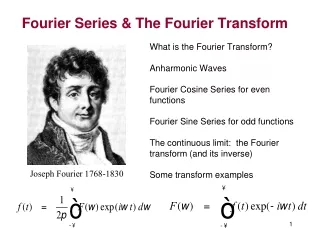
1. Theory – 1.1. Central Slice Theorem (CST)– 1.1.1 Continuous Time Fourier Transform (CTFT) - > DiscreteTime Fourier Transform (DTFT) -> Discrete Fourier Transform (DFT) -> Fast Fourier Transform (FFT) • CTFT -> DTFT Description: DTFT is a discrete time sampling version of CTFT Reasons: fast and save memory space • DTFT -> DFT Description: DFT is a discrete frequency sampling version of DTFT Reasons: fast and save memory space sampling all frequencies are not possible • DFT -> FFT Description: Faster version of FFT Reasons: even faster
1. Theory – 1.1. Central Slice Theorem (CST)– 1.1.1 CTFT - > DTFT -> DFT -> FFT Con’t • DFT -> FFT Special requirement : Number of samples should be a power of two Solution: Zeropad How to make zeropad? In the sinogram, add black lines evenly on top and bottom Physical meaning? Scan the sample in a bigger space!
1. Theory – 1.2. Interpolation Why we need interpolation? Reasons : Equal spacing for x and y coordinates are required for IF2D Reasons? • 1D Fourier Transform of Radon function is in polar coordinate • Convert to 2D Cartesian coordinate system, x = rcosq and y = rsinq Solution: Interpolation
2. Experiment –2.1. Basic – 2.1.2. Number of projection slices • As the number of projection slices decreases, the reconstructed images become blurry and have many artifacts • The resolution can be better by using more slices
2. Experiment –2.1. Basic – 2.1.2. Number of projection slices (con’t)
2. Experiment –2.1. Basic – 2.1.2. Number of projection slices (con’t)
2. Experiment –2.1. Basic– 2.1.3. Scan angle (<180, >180) • The image resolution increases as the scanning angle increases • Meanwhile artifacts reduced
2. Experiment –2.2. Advanced – 2.2.1. Noise • The noise is added on the sinogram • The more the noise, the more the data being distorted
2. Experiment –2.2. Advanced – 2.2.2. Sensor Damage • From the sinogram, each s value in the vertical axis corresponds to a sensor • If there is a sensor damaged, then it will appear as a semi-circle artifact
2. Experiment –2.2. Advanced – 2.2.2. Sensor Damage (con’t) • The more the damage sensors, the lower the quality of the reconstructed images Could we … • Replace those sensors? Definitely yes! 2. Scan the object by 360o instead of 180o? No.
3. Conclusion • Direct Fourier Reconstruction uses short computation time to give a good quality image, with all details in the Phantom can be conserved • The resolution is high and even there is little artifact, it is still acceptable. • To make the reconstructed images better, we can • use more sensors • use more projection slices • scan the Phantom more than 180o • add filters to eliminate noise • Replaced all damaged sensors.
4. Reference 1. Yao Wang, 2007, Computed Tomography, Polytechnic University 2. Forrest Sheng Bao, 2008, FT, STFT, DTFT, DFT and FFT, revisited, Forrest Sheng Bao, http://narnia.cs.ttu.edu/drupal/node/46