Download
1 / 27
280 likes | 333 Vues
Learn basics of vector calculus including vector operations, scalar and vector products, time derivatives and integrals of vector functions. Example problems and their solutions included.

E N D
Physics for informatics Lecture 1Introduction, vector calculus, functions of more variables, Ing. Jaroslav Jíra, CSc.
Introduction Lecturers: prof. Ing. Stanislav Pekárek, CSc., pekarek@fel.cvut.cz , room 49A Ing. Jaroslav Jíra, CSc., jira@fel.cvut.cz , room 42 Source of information:http://aldebaran.feld.cvut.cz/ , section Physics for OI Textbooks:Physics I, Pekárek S., Murla M. Physics I - seminars, Pekárek S., Murla M. Internet tests:https://fyzika.feld.cvut.cz/auth/oitest
Scoring system of the Physics for OI The maximum reachable amount of points from semester is 100. Points from semester go with each student to the exam, where they create a part of the final grade according to the exam rules. Conditions for assessment: - to gain at least 40 points, - to measure six laboratory experiments and submit reports from them Points can be gained by: - written tests, max. 50 points. Two tests by 25 points max. (8th and 13th week) - laboratory reports, max. 30 points. The last five lab reports are marked by up to 6 points each - tests on the internet, max. 20 points. There are 10 electronical tests available on the internet, each consisting of 8 questions. Correct answering of ALL eight questions results in 2 point gain for the student.
Examination – first part: Every student must solve certain number ofproblems according to his/herpoints from the semester.
Examination - second part: Student answers questions in written form during the written exam. The answers are marked and the total of 30 points can be gained this way. Then the oral part of the exam follows and each student defends a mark according to the table below. The column resulting in better mark is taken into account.
Vector calculus - basics A vector – standard notation for three dimensions Unit vectors i,j,kare vectors of magnitude 1 in directions of the x,y,z axes. Magnitude of a vector Position vector is a vector r from the origin to the current position where x,y,z, are projections of r to the coordinate axes.
Adding and subtracting vectors Multiplying a vector by a scalar Example of multiplying of a vector by a scalar in a plane
Example of addition of three vectors in a plane The vectors are given: Numerical addition gives us Graphical solution:
Example of subtraction of two vectors a plane The vectors are given: Numerical subtraction gives us Graphical solution:
Example of the time derivation of a vector The motion of a particle is described by the vector equation Determine for any time t: a) b) the tangential and the radial accelerations
Time derivation of a vector in the Mathematica -continued What would happen without Assuming and Refine What would happen without Simplify Graphical output of the
Example of the time integration of a vector Evaluate the time dependence of the velocity and the position vector for the projectile motion. Initial velocity v0=(10,20) m/s and g=(0,-9.81) m/s2.
Time integration of a vector in the Mathematica Study of balistic projectile motion, whencomponents of initial velocity are given Projectile motion - trajectory:
Scalar product Scalar product (dot product) – is defined as Where Θ is a smaller angle between vectors a and b and S is a resulting scalar. For three component vectors we can write Geometric interpretation – scalar product is equal to the area of rectangle havinga and b.cosΘas sides.Blue and red arrows represent original vectors a and b. Basic properties of the scalar product
Vector product Vector product (cross product) – is defined as Where Θ is the smaller angle between vectors a and b and n is unit vector perpendicular to the plane containing a and b. Geometric interpretation - the magnitude of the cross product can be interpreted as the positive area Aof the parallelogram having a and b as sides Component notation Basic properties of the vector product
Direction of the resulting vector of the vector productcan be determined eitherby the right hand rule or by the screw rule Vector triple product Geometric interpretation of the scalar triple product isa volume of a paralellepipedV Scalar triple product
Scalar field and gradient Scalar fieldassociates a scalar quantity to every point in a space. This association can be described by a scalar function fand can be also time dependent. (for instance temperature, density or pressure distribution). The gradient of a scalar field is a vector field that points in the direction of the greatest rate of increase of the scalar field, and whose magnitude is that rate of increase. Example: the gradient of the function f(x,y) = −(cos2x + cos2y)2 depicted as a projected vector field on the bottom plane.
Example 2 – finding extremes of the scalar field Find extremes ofthe function: Extremes can be found by assuming: In this case : Answer: there are two extremes
Vector operators Gradient (Nabla operator) Divergence Curl Laplacian