Download
1 / 29
330 likes | 638 Vues
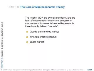
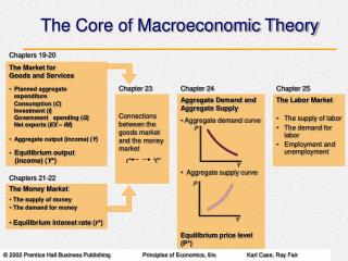
The Core of Macroeconomic Theory. Aggregate Output and Aggregate Income ( Y ). Aggregate output is the total quantity of goods and services produced (or supplied) in an economy in a given period. Aggregate income is the total income received by all factors of production in a given period.

E N D
Aggregate Output andAggregate Income (Y) • Aggregate output is the total quantity of goods and services produced (or supplied) in an economy in a given period. • Aggregate income is the total income received by all factors of production in a given period.
Aggregate Output andAggregate Income (Y) • Aggregate output (income) (Y) is a combined term used to remind you of the exact equality between aggregate output and aggregate income. • When we talk about output (Y), we mean real output, not nominal output. Output refers to the quantities of goods and services produced, not the dollars in circulation.
Income, Consumption,and Saving (Y, C, and S) • A household can do two, and only two, things with its income: It can buy goods and services—that is, it can consume—or it can save. • Saving is the part of its income that a household does not consume in a given period. Distinguished from savings, which is the current stock of accumulated saving.
Saving / Aggregate Income - Consumption • All income is either spent on consumption or saved in an economy in which there are no taxes.
Explaining Spending Behavior • Some determinants of aggregate consumption include: • Household income • Household wealth • Interest rates • Households’ expectations about the future • In The General Theory, Keynes argued that household consumption is directly related to its income.
A Consumption Functionfor a Household • The relationship between consumption and income is called the consumption function. • The consumption function for an individual household shows the level of consumption at each level of household income.
An Aggregate Consumption Function • For simplicity, we assume that points of aggregate consumption, when plotted against aggregate income, lie along a straight line. • The slope of the consumption function (b) is called the marginal propensity to consume (MPC), or the fraction of a change in income that is consumed, or spent.
An Aggregate Consumption FunctionDerived from the Equation C = 100 + .75Y • At a national income of zero, consumption is $100 billion (a). • For every $100 billion increase in income (DY), consumption rises by $75 billion (DC).
An Aggregate Consumption FunctionDerived from the Equation C = 100 + .75Y
Consumption and Saving • Since there are only two places income can go: consumption or saving, the fraction of additional income that is not consumed is the fraction saved. The fraction of a change in income that is saved is called the marginal propensity to save (MPS). • Once we know how much consumption will result from a given level of income, we know how much saving there will be. Therefore,
Planned Investment (I) • Investment refers to purchases by firms of new buildings and equipment and additions to inventories, all of which add to firms’ capital stocks. • One component of investment—inventory change—is partly determined by how much households decide to buy, which is not under the complete control of firms. change in inventory = production – sales
Planned Investment (I) • Desired or planned investment refers to the additions to capital stock and inventory that are planned by firms. • Actual investment is the actual amount of investment that takes place; it includes items such as unplanned changes in inventories.
Planned Investment (I) • For now, we will assume that planned investment is fixed. It does not change when income changes. • When a variable, such as planned investment, is assumed not to depend on the state of the economy, it is said to be an autonomous variable.
Planned Aggregate Expenditure (AE) • To determine planned aggregate expenditure (AE), we add consumption spending (C) to planned investment spending (I) at every level of income.
Equilibrium Aggregate Output (Income) • In macroeconomics, equilibrium in the goods market is the point at which planned aggregate expenditure is equal to aggregate output.
Equilibrium Aggregate Output (Income) aggregate output /Yplanned aggregate expenditure /AE/C + Iequilibrium: Y = AE, or Y = C + I Disequilibria: Y > C + I aggregate output > planned aggregate expenditureInventory investment is greater than planned.Actual investment is greater than planned investment. C + I > Yplanned aggregate expenditure > aggregate outputInventory investment is smaller than planned.There is unplanned inventory disinvestment.
(1) (2) (3) Finding EquilibriumOutput Algebraically There is only one value of Y for which this statement is true. We can find it by rearranging terms: By substituting (2) and (3) into (1) we get:
The Saving/InvestmentApproach to Equilibrium Saving is a leakage out of the spending stream. If planned investment is exactly equal to saving, then planned aggregate expenditure is exactly equal to aggregate output, and there is equilibrium.
The S = I Approach to Equilibrium • Aggregate output will be equal to planned aggregate expenditure only when saving equals planned investment (S = I).
The Multiplier • The multiplier is the ratio of the change in the equilibrium level of output to a change in some autonomous variable. • An autonomous variable is a variable that is assumed not to depend on the state of the economy—that is, it does not change when the economy changes. • In this chapter, for example, we consider planned investment to be autonomous.
The Multiplier • An increase in planned investment causes output to go up. People earn more income, consume some of it, and save the rest. • The multiplier of autonomous investment describes the impact of an initial increase in planned investment on production, income, consumption spending, and equilibrium income.
The Multiplier • The size of the multiplier depends on the slope of the planned aggregate expenditure line. • The marginal propensity to save may be expressed as: • Because DS must be equal to DI for equilibrium to be restored, we can substitute DI for DS and solve: therefore, , or
The Multiplier • After an increase in planned investment, equilibrium output is four times the amount of the increase in planned investment.
The Multiplier • In reality, the size of the multiplier is about 1.4. That is, a sustained increase in autonomous spending of $10 billion into the U.S. economy can be expected to raise real GDP over time by $14 billion.
The Paradox of Thrift • When households are concerned about the future and plan to save more, the corresponding decrease in consumption leads to a drop in spending and income. • In their attempt to save more, households have caused a contraction in output, and thus in income. They end up consuming less, but they have not saved any more.