What is a slice?
Learn about dynamic and static slicing to analyze program dependencies. Explore applications, examples, issues, and efficiency considerations. Discover various algorithms and strategies for efficient slicing computation.

What is a slice?
E N D
Presentation Transcript
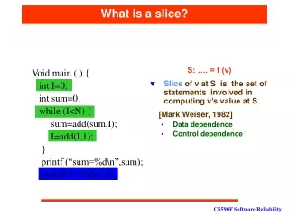
What is a slice? S: …. = f (v) • Slice of v at S is the set of statements involved in computing v’s value at S. [Mark Weiser, 1982] • Data dependence • Control dependence Void main ( ) { int I=0; int sum=0; while (I<N) { sum=add(sum,I); I=add(I,1); } printf (“sum=%d\n”,sum); printf(“I=%d\n”,I);
Static Slicing Static slice is the set of statements that COULD influence the value of a variable for ANY input. • Construct static dependence graph • Control dependences • Data dependences • Traverse dependence graph to compute slice • Transitive closure over control and data dependences
Dynamic Slicing Dynamic slice is the set of statements that DID affect the value of a variable at a program point for ONE specific execution. [Korel and Laski, 1988] • Execution trace • control flow trace -- dynamic control dependences • memory reference trace -- dynamic data dependences • Construct a dynamic dependence graph • Traverse dynamic dependence graph to compute slices • Smaller, more precise, slices are more helpful
Static slice can be much larger than the dynamic slice Slice Sizes: Static vs. Dynamic
Applications of Dynamic Slicing • Debugging [Korel & Laski - 1988] • Detecting Spyware [Jha - 2003] • Installed without users’ knowledge • Software Testing [Duesterwald, Gupta, & Soffa - 1992] • Dependence based structural testing - output slices. • Module Cohesion [N.Gupta & Rao - 2001] • Guide program structuring • Performance Enhancing Transformations • Instruction criticality [Ziles & Sohi - 2000] • Instruction isomorphism [Sazeides - 2003] • Others…
Dynamic Slicing Example -background For input N=2, 11: b=0 [b=0] 21: a=2 31: for i = 1 to N do [i=1] 41: if ( (i++) %2 == 1) then [i=1] 51: a=a+1 [a=3] 32: for i=1 to N do [i=2] 42: if ( i%2 == 1) then [i=2] 61: b=a*2 [b=6] 71: z=a+b [z=9] 81: print(z) [z=9] 1: b=0 2: a=2 3: for i= 1 to N do 4: if ((i++)%2==1) then 5: a = a+1 else 6: b = a*2 endif done 7: z = a+b 8: print(z)
Issues about Dynamic Slicing • Precision – perfect • Running history – very big ( GB ) • Algorithm to compute dynamic slice - slow and very high space requirement.
Efficiency • How are dynamic slices computed? • Execution traces • control flow trace -- dynamic control dependences • memory reference trace -- dynamic data dependences • Construct a dynamic dependence graph • Traverse dynamic dependence graph to compute slices
Graphs of realistic program runs do not fit in memory. The Graph Size Problem
Conventional Approaches • [Agrawal &Horgan, 1990] presented three algorithms to trade-off the cost with precision. Algo.I Algo.II Algo.III Precise dynamic analysis Static Analysis high Cost: low Precision: low high
Algorithm One • This algorithm uses a static dependence graph in which all executed nodes are marked dynamically so that during slicing when the graph is traversed, nodes that are not marked are avoided as they cannot be a part of the dynamic slice. • Limited dynamic information - fast, imprecise (but more precise than static slicing)
11 21 31 41 51 71 81 Algorithm I Example 1: b=0 For input N=1, the trace is: 2: a=2 3: 1 <=i <=N T 4: if ((i++)%2= =1) F T F 5: a=a+1 6: b=a*2 32 7: z=a+b 8: print(z)
Algorithm I Example 1: b=0 2: a=2 DS={1,2,5,7,8} 3: 1 <=i <=N Precise! 4: if ((i++)%2= =1) 5: a=a+1 6: b=a*2 7: z=a+b 8: print(z)
Imprecision introduced by Algorithm I Input N=2: for (a=1; a<N; a++) { … if (a % 2== 1) { b=1; } if (a % 3 ==1) { b= 2* b; } else { c=2*b+1; } } 4 1 2 3 4 5 6 7 8 9 7 9 Killed definition counted as reaching!
Algorithm II • A dependence edge is introduced from a load to a store if during execution, at least once, the value stored by the store is indeed read by the load (mark dependence edge) • No static analysis is needed.
11 21 31 41 51 71 81 Algorithm II Example 1: b=0 For input N=1, the trace is: 2: a=2 3: 1 <=i <=N T 4: if ((i++)%2= =1) F T F 5: a=a+1 6: b=a*2 7: z=a+b 8: print(z)
Algorithm II – Compare to Algorithm I • More precise Algo. II Algo. I x=… x=… …=x …=x …=x …=x
Efficiency: Summary • For an execution of 130M instructions: • space requirement: reduced from 1.5GB to 94MB (I further reduced the size by a factor of 5 by designing a generic compression technique [MICRO’05]). • time requirement: reduced from >10 Mins to <30 seconds.
Algorithm III • First preprocess the execution trace and introduces labeled dependence edges in the dependence graph. During slicing the instance labels are used to traverse only relevant edges.
Dynamic Dep. Graph Representation N=2: 1: sum=0 2: i=1 1: sum=0 2: i=1 3: while ( i<N) do 3: while ( i<N) do 4: i=i+1 5: sum=sum+i 4: i=i+1 5: sum=sum+i 3: while ( i<N) do 4: i=i+1 5: sum=sum+i 6: print (sum) 3: while ( i<N) do 6: print (sum)
Dynamic Dep. Graph Representation Timestamps N=2: 1: sum=0 2: i=1 1: sum=0 2: i=1 0 0 1 1 3: while ( i<N) do 3: while ( i<N) do 4: i=i+1 5: sum=sum+i 2 2 4: i=i+1 5: sum=sum+i (2,2) (4,4) 3 3 3: while ( i<N) do 4: i=i+1 5: sum=sum+i (4,6) 4 4 6: print (sum) 5 5 3: while ( i<N) do 6 6 6: print (sum) • A dynamic dep. edge is represented as by an edge annotated with a pair of timestamps <definition timestamp, use timestamp>
(...,20) ... X = X = X = (10,10) (20,20) (30,30) Y= X Y= X Y= X (20,21) ... =Y 21 Infer: Local Dependence Labels: Full Elimination 10,20,30
X = X = X = (20,20) *P = *P = *P = (10,10) Y= X Y= X Y= X =Y 11,21 Transform: Local Dependence Labels: Elimination In Presence of Aliasing (20,21) ... 10,20
X = X = X = X = (20,20) *P = *P = *P = *P = (10,10) Y= X Y= X Y= X Y= X (10,11) (20,21) (10,11) (20,21) =Y =Y 11,21 11,21 Transform: Local Dependence Labels: Elimination In Presence of Aliasing 10 20 10,20
1 1 1 1 1 2 2 2 2 2 3 3 3 3 4 6 7 9 3 4 6 7 9 3 5 6 7 9 3 4 6 8 9 3 5 6 8 9 4 4 5 5 4 3 3 6 6 5 6 7 8 7 8 9 9 7 10 10 Transform: Coalescing Multiple Nodes into One 1 2 10
X = Y = X = Y = X = Y = (10,21) X = Y = X = Y = X = Y = (10,21) (10,21) (20,11) (20,11) = Y = X = Y = X = Y = X (20,11) Group: Labels Across Non-Local Dependence Edges 10 20 11,21