Download
1 / 31
310 likes | 486 Vues
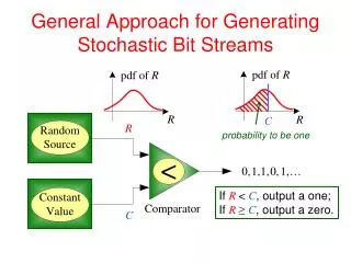
General Approach for Generating Stochastic Bit Streams. R. probability to be one. 0,. 1,. 1,. 0,. 1,. …. If R < C , output a one; If R ≥ C , output a zero. Comparator. C. Types of Random Sources. Psuedorandom Number Generator. Linear Feedback Shift Register. (expensive).

E N D
General Approach for Generating Stochastic Bit Streams R probability to be one 0, 1, 1, 0, 1, … If R < C, output a one; If R ≥ C, output a zero. Comparator C
Types of Random Sources • Psuedorandom Number Generator Linear Feedback Shift Register (expensive) • Physical Random Source Thermal Noises (cheap)
Challenge withPhysical Random Sources cheap Voltage Regulators expensive expensive C2 C1 Suppose many differentprobabilities are needed:{0.2, 0.78, 0.2549, 0.43, 0.671, 0.012, 0.82, …}. It is costly to generate them directly.(many expensive constant values required.)
Opportunity with Physical Random Sources cheap 1,1,0,0,0, … 0,1,0,1,0, … 0,0,1,0,1, … expensive • Independent • Same probability
Solution When we need many different probabilities: {0.2, 0.78, 0.2549, 0.43, 0.671, 0.012, 0.82, …} • Generate a few probabilities directly from physical random sources. • Synthesize combinational logic to generate other probabilities. Probability: Probability of a signal being logical one
Basic Problem Other Probabilities Needed Set S of Input Probabilities(|S| small) p1 q1 q2 p2 q3 p3 q4 RandomSources LogicCircuit • Synthesize Logic Circuit? • Choose Set S?
Assumptions • All signals in the circuit are random Boolean variables. • Elements of set S can be used many times. • All inputs are independent. p1 p1 p2 logiccircuit p2 q p3 p3 Independent p3
Conventions • “Probability”: Probability of a signal being logical one • “Synthesize probability q”: Synthesize the circuit generating probability q
Example 0.6 0.4 0.2 0.5 0.3 P(x = 1) = 0.4 P(x = 1) = 0.4 0,0,1,0,1,0,1,0,1,0 0,1,0,1,0,0,1,1,0,0 P(z = 1) = 0.3 P(z = 1) = 0.2 P(z = 1) = 0.6 P(x = 1) = 0.4 0,1,0,0,0,1,0,0,0,1 0,0,0,1,0,0,1,0,0,0 LogicCircuit 1,0,1,1,0,1,0,0,0,0 0,1,0,0,1,0,1,1,1,1 1,0,0,1,1,0,0,1,1,0 1,0,1,1,0,0,1,0,0,1 P(y = 1) = 0.5 P(y = 1) = 0.5 P(z = 1) = P(x = 0) P(z = 1) = P(x = 0) P(y = 0) P(z = 1) = P(x = 1) P(y = 1)
Generating Decimal Probabilities Decimal Probabilities Choose Set S = {p1, p2, p3} p1 q1 p2 q2 q3 p3 q4 LogicCircuit Large Cost! |S| Small! • Found Set S for • |S| = 2 • |S| = 1
Generating Decimal Probabilities Theorem 1: With S = {0.4, 0.5}, we can synthesize arbitrarydecimal output probabilities. Example: Synthesize q = 0.757 (Black dots are inverters)
Proof of Theorem 1 • Constrain design to AND gates and inverters • AND gates: x ∙ y • Inverters: 1 − x • Constructive proof • Induction on the number of digits n • Base case • 0.1 = 0.4 × 0.5 × 0.5 0.9 = 1 − 0.1 • 0.2 = 0.4 × 0.5 0.8 = 1 − 0.2 • 0.3 = (1 − 0.4) × 0.5 0.7 = 1 − 0.3 • 0.6 = 1 − 0.4 • Inductive step • Assume true for (n − 1). Show true forn.
Proof of Inductive Step q: n digits; w: (n−1) digits; u = 10nq, numerator of q conversions cases w = 5qq = 0.4 × 0.5 × w 0 ≤ q ≤ 0.2, u = 2k w = 10qq = 0.4×0.5×0.5×w 0 ≤ q ≤ 0.1, u = 2k+1 w = 2 − 10qq = (1−0.5w)×0.4×0.5 q 0.1 < q ≤ 0.2, u = 2k+1 w = 2.5qq = 0.4 × w 0.2 < q ≤ 0.4, u = 4k …
Algorithm from Theorem 1 Example: Synthesize q = 0.757 from S= {0.4, 0.5} 1 − ×0.4 1 − ×0.5 1 − ×0.5 0.757 0.243 0.6075 0.43 0.3925 0.785 0.215 1 − ×0.5 1 − ×0.5 1 − ×0.5 ×0.4 0.86 0.14 0.6 0.3 0.35 0.4 0.7 Base case cases conversions 0 ≤ q ≤ 0.2, u = 2k w = 5q 0 ≤ q ≤ 0.1, u = 2k+1 w = 10q … … 0.2 < q ≤ 0.3, u = 2k+1 w = 10q − 2 0.3 < q ≤ 0.4, u = 2k+1 w = 4 − 10q 0.4 < q ≤ 0.5 w = 1 − 2q 0.5 < q ≤ 1 w = 1− q
Circuit Synthesized (Black dots are inverters) 1 − ×0.4 1 − ×0.5 1 − ×0.5 0.6075 0.43 0.3925 0.785 0.215 0.757 0.243 1 − ×0.5 1 − ×0.5 1 − ×0.5 ×0.4 0.14 0.86 0.4 0.6 0.3 0.7 0.35
combinationalcircuit Generating Decimal Probabilities Question: Does there exist a set S of size one which can generate arbitrary decimal probabilities? p p Independent q p p Yes!
Proof • There exists a p (≈ 0.1295) in the unit interval such that • Boolean function with , has output probability • Boolean function with , has output probability • Thus, 0.4 and 0.5 can be generated from p. (Use • Theorem 1.)
Implementation • Focus on generating decimal probability formS = {0.4, 0.5}. • Goal: Reduce circuit depth.
Balancing • Logic Level Optimization: Balancing After Balancing Before Balancing (a and b are primary inputs)
Factorization of Fractions • High Level Optimization: Factorization of Fractions Example: Synthesize q = 0.49 from S = {0.4, 0.5} Basic Factor
Factorization of Fractions • Quality of factor pair a = al × ar • Heuristic: Digits(x) ↑Depth of the circuit for fraction x↑ • Measure for depth: Max{Digits(al), Digits (ar)} + 1
Factorization of Fractions Example: 0.1764 = 0.252×0.7 =0.63×0.28 better!
Factorization of Fractions • Consider both q and 1 − q • Example: q = 0.37, then 1 − q = 0.63 has better factor pair 0.7×0.9 • When both q and 1 − q cannot be factorized • Use conversions from Theorem 1 to get w with one less digit than q. • Factorize w.
Experimental Results • ‘Basic’: Algorithm based on Theorem 1 + Balancing • ‘Factor’: Algorithm based on Factorization + Balancing • Compare number of AND gates and depth of synthesized circuits • Present average results for different numbers of digits n
Experimental Results Average number of AND gates vs. number of digits n
Experimental Results Average depth vs. number of digits n
Summary • Considered the problem of generating required decimal probabilities. • Gave a pair of probabilities / a single probability for generating arbitrary decimal probabilities. • Proposed implementation based on balancing and factorization of fractions to reduce the depth of the circuit. • Also considered synthesis with different assumptions: • Whether the probabilities are duplicable or not. • Whether we are free to choose input probability set.
Precision versus Bit Length • Stochastic encoding • Uniform and not compact: To represent 2n different values, need 2n bits • Binary radix encoding • Positional and compact: To represent 2n different values, need n bits For applications that can tolerate small error, we don’t need a large n.
Error due to Stochastic Variance • x = P(X = 1) = 2/5 → 0,1,0,1,1 (x= 3/5) • Increasing the length of bit streams reduces the error. • Effect of errors is uniform and small. • Target application: low precision, e.g., hardware for sensing appication operating in harsh environments.
Comparison of Encoding (Positional, Weighted) (Uniform) (Uniform,Long Stream) (Positional) (Compact, Efficient) (Not compact, Long Stream) Binary Radix Encoding Stochastic Encoding Spectrum of Encoding
Future Directions Spectrum of Encoding ? Binary Radix Encoding(Compact, Positional) Stochastic Encoding (Not compact, Uniform) Possible encodings in the middle with theadvantages of both?