Download
1 / 70
700 likes | 835 Vues
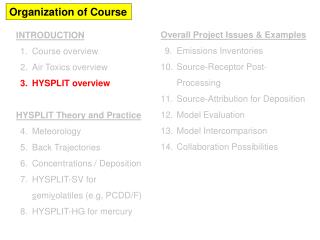
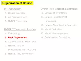
Organization of Course. Overall Project Issues & Examples Emissions Inventories Source-Receptor Post-Processing Source-Attribution for Deposition Model Evaluation Model Intercomparison Collaboration Possibilities. INTRODUCTION Course overview Air Toxics overview HYSPLIT overview

E N D
Organization of Course Overall Project Issues & Examples Emissions Inventories Source-Receptor Post-Processing Source-Attribution for Deposition Model Evaluation Model Intercomparison Collaboration Possibilities INTRODUCTION Course overview Air Toxics overview HYSPLIT overview HYSPLIT Theory and Practice Meteorology Back Trajectories Concentrations / Deposition HYSPLIT-SV for semivolatiles (e.g, PCDD/F) HYSPLIT-HG for mercury
“Hands On” HYSPLIT Modeling Exercise #1 Running and Mapping a Single Back-Trajectory using the Graphical User Interface (GUI)
First, delete all files from “c:\hysplit4\working” Second, copy all files from “c:\hysplit4\working_start” into “c:\hysplit4\working”
“Starting time”: change to 08 08 03 15 “Total run time”: change to -24 1 Change to: 20.25 -103.05 200 2 6 -24 7 Click “OK” Click “Setup starting locations” 5 “Direction”: change to ”Back” 3 “Number of starting locations”: change to 1 4
Click “Clear” to remove Oct1618.bin 8 Click “Add Meteorology Files” 9 Navigate to folder c:\hysplit4\metdata 10 double click on the file: edas.aug08.001 11 When everything looks like the above, click “Save” 13 Then double click on the file: edas.jul08.002 12
click “Trajectory” 14 click “Run Model” 15 When simulation is complete, click “Exit” 16
Select Time Label Interval (UTC) = 1 Select Vertical Coordinate = “Meters –agl” Click “Execute Display”
If there is time, we can vary the trajectory setup (and then rerun the trajectory) and/or vary the trajectory display features and look at how the trajectory changes…
What does the Graphical User Interface (GUI) actually do? • Writes a “control” file • and other input files as needed, setup.cfg • Runs the HYSPLIT Trajectory Model • which reads the control file and other input files • Runs the “Trajplot” Display Program, according to the user’s preferences
“Hands On” HYSPLIT Modeling Exercise #2 Running and Mapping a Single Back-Trajectory from the DOS Command Line
If a CONTROL file is present in the working directory, then HYSPLIT will read it and run a trajectory according to this file’s specifications starting year, month, day, hour (UTC) -- number of starting locations -- lat, long, height (m-agl) for each location -- hours to run trajectory (if < 0, then backward) -- vertical motion option (0:data, …) -- model top (meters) -- number of meteorological data files to use -- location of first file -- name of first file -- location of next file -- name of next file -- location of output (./ = working directory) -- name of trajectory endpoints file -- 08 08 03 15 1 20.25 -103.05 200.0 -24 0 10000.0 2 C:/hysplit4/metdata/ edas.aug08.001 C:/hysplit4/metdata/ edas.jul08.002 ./ tdump
Open a DOS Command Prompt Window: • Start, All Programs, Accessories, Command Prompt • Navigate to c:\hysplit4\working_02: • cd\ [enter] • cd c:\hysplit4\working_02 [enter] • dir [enter] • The files in this • directory are equivalent to the files that were just created in the working directory by our actions with the GUI • The files were copied for you to this new folder for the next exercise
Run the HYSPLIT Trajectory program by typing: • ..\exec\hyts_std [enter] • HYSPLIT runs! • Display files in directory: • dir [enter] • There are two new files: • MESSAGE • tdump
Starting time Starting location hour lat long height pressure
Invoke TRAJPLOT.exe trajectory mapping program with no arguments to see its “USAGE” • ..\exec\trajplot [enter]
Now run TRAJPLOT.exe program “for real” with a few simple arguments: • ..\exec\trajplot –a3 –v1 -itdump [enter] -a3 gives Google Earth KML file output -v1 gives vertical output in meters above ground level -itdump tells program to use tdump as the trajectory endpoints file
There are two new files present: • Trajplot.ps • HYSPLITtraj_ps_01.kml
Now Double Click on KML file, if Google Earth has been installed
You can see this can all be • done from the Command Line • It can also be done using a DOS Batch File Has anyone had experience using DOS Batch Files?
“Hands On” HYSPLIT Modeling Exercise #3 Running and Mapping a Single Back-Trajectory with a DOS Batch File
TRAJ_RUN_03.bat @ECHO OFF rem starting time ECHO 08 08 03 15 > CONTROL.txt rem number of starting locations ECHO 1 >> CONTROL.txt rem lat, long, height of start location ECHO 20.25 -103.05 200.0 >> CONTROL.txt rem number of hours to run trajectory ECHO -24 >> CONTROL.txt rem vertical motion option rem (0:data 1:isob 2:isen 3:dens 4:sigma 5:diverg 6:eta) ECHO 0 >> CONTROL.txt rem model top ECHO 10000.0 >> CONTROL.txt rem number of meteorological data files ECHO 2 >> CONTROL.txt rem location and name of first met file ECHO C:/hysplit4/metdata/ >> CONTROL.txt ECHO edas.aug08.001 >> CONTROL.txt rem location and name of second met file ECHO C:/hysplit4/metdata/ >> CONTROL.txt ECHO edas.jul08.002 >> CONTROL.txt rem location and name of trajectory endpoints output file ECHO ./ >> CONTROL.txt ECHO tdump >> CONTROL.txt
TRAJ_RUN_03.bat (continued) rem delete earlier CONTROL if present del CONTROL. rem copy new file to "control" copy CONTROL.txt control. rem run hysplit trajectory model (it will use "control." ..\exec\hyts_std.exe rem run trajplot to map the trajectory ..\exec\trajplot -itdump -a3 –v1
“Hands On” HYSPLIT Modeling Exercise #4 Running and Mapping a Single Back-Trajectory with a DOS Batch File with Replaceable Parameters
TRAJ_SET_04.bat @ECHO OFF rem parameter #1: start year (UTC) rem parameter #2: start month (UTC) rem parameter #3: start day (UTC) rem parameter #4: start hour (UTC) rem parameter #5: run name rem parameter #6: metfile_1 rem parameter #7: metfile_2 rem parameter #8: metfile_3 rem starting time ECHO %1 %2 %3 %4 > CONTROL.txt rem number of starting locations ECHO 1 >> CONTROL.txt rem lat, long, height of start location ECHO 20.25 -103.05 200.0 >> CONTROL.txt rem number of hours to run trajectory ECHO -24 >> CONTROL.txt rem vertical motion option rem (0:data 1:isob 2:isen 3:dens 4:sigma 5:diverg 6:eta) ECHO 0 >> CONTROL.txt rem model top ECHO 10000.0 >> CONTROL.txt
TRAJ_SET_04.bat … continued rem number of meteorological data files ECHO 3 >> CONTROL.txt rem location and name of first met file ECHO C:/hysplit4/metdata/ >> CONTROL.txt ECHO %6 >> CONTROL.txt rem location and name of second met file ECHO C:/hysplit4/metdata/ >> CONTROL.txt ECHO %7 >> CONTROL.txt rem location and name of third met file ECHO C:/hysplit4/metdata/ >> CONTROL.txt ECHO %8 >> CONTROL.txt rem location and name of trajectory endpoints output file ECHO ./ >> CONTROL.txt ECHO tdump.txt >> CONTROL.txt rem delete earlier CONTROL if present del CONTROL. rem copy new file to "control" rename CONTROL.txt control. rem run hysplit trajectory model, using "control." ..\exec\hyts_std.exe rem run trajplot to map the trajectory ..\exec\trajplot -itdump -a3 –v1
TRAJ_SET_04.bat … continued rem now rename all files with run name identifier rename tdump.txt %5.tdp rename message. %5.msg rename trajplot.ps %5.ps rename control. %5.ctl rename HYSPLITtraj_ps_01.kml %5.kml rename TRAJ.CFG %5.cfg rem now create folder for key files mkdir temp rem now move all key files into this folder move %5.* temp rem now rename folder to run name rename temp %5
TRAJ_RUN_04.bat • call TRAJ_SET_04 • 08 03 15 • LC_UTC_2008_08_03_15 • edas.jul08.002 • edas.aug08.001 • edas.aug08.002 Start day Start hour Start year Start month Meteorological data file #2 “run name” call TRAJ_SET_04 08 08 03 15 LC_n0001_UTC_2008_08_03_15 edas.jul08.002 edas.aug08.001 edas.aug08.002 Meteorological data file #1 Meteorological data file #3 TRAJ_SET_04 is the batch file we were just discussing It is “called” from the batch file: TRAJ_RUN_04.bat
Type “TRAJ_RUN_04” at the command prompt in working_04, and the batch file does everything!
Greater than ~20km from the source, if the forward trajectory from the source is within the PBL, then the source can impact the measurement site, even if the trajectory endpoint near the site is not at the height of the sampler… This is because the PBL is relatively well-mixed during the day. Height of Planetary Boundary Layer (PBL) During the Day • a forward trajectory is the “center line” of a plume • horizontal & vertical dispersion around this center line Measurement of ambient air concentrations
At night, the Planetary Boundary Layer (PBL) is generally much shallower • Emissions from an elevated stack may be emitted above the PBL • In this case, little or no impact on a ground-based measurement site until the next daytime period, when the boundary layer grows. Height of Planetary Boundary Layer (PBL) At Night Measurement of ambient air concentrations
At night, the Planetary Boundary Layer (PBL) is generally much shallower • Emissions from an relatively low stack may be emitted within the PBL • But, if the pollutant dry deposits relatively rapidly (e.g., reactive gaseous mercury (“RGM”), by the time the plume reaches the receptor, there may be little pollutant left… Height of Planetary Boundary Layer (PBL) At Night dry deposition can deplete near-ground plume Measurement of ambient air concentrations
What are the implications of these ideas for back-trajectories? • What HEIGHT should one start a back-trajectory? • If you start very low to the ground, at the sampler height, the trajectory program does not work well… the trajectories hit the ground and stop • “best” starting height for back-trajectories may be from the middle of the Planetary Boundary Layer PBL Height H = 0.5 * PBL Measurement of ambient air concentrations
“Hands On” HYSPLIT Modeling Exercise #5 Running and Mapping a Multiple Back-Trajectories with a DOS Batch File with Replaceable Parameters with variations in the SETUP.CFG file, e.g., specifying starting height as fraction of the Planetary Boundary Layer
IF SETUP.CFG Namelist file is present, then HYSPLIT will use it. • If not, then HYSPLIT will just use DEFAULT values for these parameters • The SETUP.CFG file contains parameters that are less frequently changed, as opposed to the CONTROL file which contains more basic run information setup_cfg_frac_pbl.txt &SETUP KMSL=2 / We will add the following statement into the “set” batch file: copy setup_cfg_frac_pbl.txt setup.cfg And then specify heights as fraction of boundary layer, e.g., 0.5
These are new elements of the TRAJ_SET file, now in TRAJ_SET_05.bat The rest of the batch file is essentially the same del setup.cfg copy setup_cfg_frac_pbl.txt setup.cfg rem starting time ECHO %1 %2 %3 %4 > CONTROL.txt rem number of starting locations ECHO 5 >> CONTROL.txt rem lat, long, fraction pbl of each start location ECHO 20.25 -103.05 0.1 >> CONTROL.txt ECHO 20.25 -103.05 0.3 >> CONTROL.txt ECHO 20.25 -103.05 0.5 >> CONTROL.txt ECHO 20.25 -103.05 0.7 >> CONTROL.txt ECHO 20.25 -103.05 0.9 >> CONTROL.txt The “run” batch file that calls this “set” file is the same