Final Exam
Prepare for the final exam on August 7, 2014, from 19:00 to 22:00. This closed-book exam will cover the entire course with a focus on topics like hash tables, binary search trees, sorting, and graphs. Key study strategies include reviewing lecture slides, reading the textbook, practicing with provided problems, and revisiting midterm solutions. Important topics include binary search tree operations (insertion, deletion), AVL trees, and search algorithms. Ensure you practice writing clear pseudocode and feel free to reach out via email or Skype for assistance.


Final Exam
E N D
Presentation Transcript
Final Exam Thursday, 7 August 2014,19:00 – 22:00 Closed Book Will cover whole course, with emphasis on material after midterm (hash tables, binary search trees, sorting, graphs)
Suggested Study Strategy Review and understand the slides. Read the textbook, especially where concepts and methods are not yet clear to you. Do all of the practice problems provided. Do extra practice problems from the textbook. Review the midterm and solutions for practice writing this kind of exam. Practice writing clear, succinct pseudocode! Review the assignments See me or one of the TAs if there is anything that is still not clear.
Assistance Regular office hours will not be held You may me by email / Skype
Summary of Topics Binary Search Trees Sorting Graphs
Binary Search Trees Insertion Deletion AVL Trees Splay Trees
A binary search tree is a binary tree storing key-value entries at its internal nodes and satisfying the following property: Let u, v, and w be three nodes such that u is in the left subtree of v and w is in the right subtree of v. We havekey(u)≤key(v)≤key(w) The textbook assumes that external nodes are ‘placeholders’: they do not store entries (makes algorithms a little simpler) An inorder traversal of a binary search trees visits the keys in increasing order Binary search trees are ideal for maps or dictionaries with ordered keys. 6 2 9 1 4 8 Binary Search Trees
Binary Search Tree • All nodes in left subtree≤ Any node ≤ All nodes in right subtree 38 ≤ ≤ ≤ 25 51 17 31 42 63 4 21 28 35 40 49 55 71
38 25 51 17 31 42 63 4 21 28 35 40 49 55 71 Search: Define Step • Cut sub-tree in half. • Determine which half the key would be in. • Keep that half. key 17 If key < root, then key is in left half. If key = root, then key is found If key > root, then key is in right half.
Insertion (For Dictionary) • To perform operation insert(k, o), we search for key k(using TreeSearch) • Suppose kis not already in the tree, and letwbe the leaf reached by the search • We insert kat node wand expand winto an internal node • Example: insert 5 w 6 6 < 2 9 2 9 > 1 4 8 1 4 8 > w 5
Insertion • Suppose kisalready in the tree, at node v. • We continue the downward search through v, and letwbe the leaf reached by the search • Note that it would be correct to go either left or right at v. We go left by convention. • We insert kat node wand expand winto an internal node • Example: insert 6 w 6 6 < 2 9 2 9 > 1 4 8 1 4 8 > w 6
Deletion • To perform operation remove(k), we search for key k • Suppose key k is in the tree, and letvbe the node storing k • If node v has a leaf child w, we remove v and w from the tree with operation removeExternal(w), which removes w and its parent • Example: remove 4 6 6 < 2 9 2 9 > v 1 4 8 1 5 8 w 5
Deletion (cont.) • Now consider the case where the key k to be removed is stored at a node v whose children are both internal • we find the internal node wthat follows v in an inorder traversal • we copy the entry stored at winto node v • we remove node wand its left child z(which must be a leaf) by means of operation removeExternal(z) • Example: remove 3 1 1 v v 3 5 2 8 2 8 6 9 6 9 w 5 z
Performance • Consider a dictionary with n items implemented by means of a binary search tree of height h • the space used is O(n) • methods find, insert and remove take O(h) time • The height h is O(n) in the worst case and O(logn) in the best case • It is thus worthwhile to balance the tree (next topic)!
AVL Trees • AVL trees are balanced. • An AVL Tree is a binary search tree in which the heights of siblings can differ by at most 1. height 0 0 0 0 0 0 0 0 0
Height of an AVL Tree • Claim: The height of an AVL tree storing n keys is O(logn).
Insertion height = 3 height = 4 7 7 Insert(2) 2 3 1 1 8 4 8 4 Problem! 1 2 1 1 0 0 0 0 5 3 5 3 1 0 0 0 0 0 0 0 2 0 0 Imbalance may occur at any ancestor of the inserted node.
Insertion: Rebalancing Strategy height = 4 7 3 1 8 4 Problem! 2 1 0 0 5 3 1 0 0 0 2 0 • Step 1: Search • Starting at the inserted node, traverse toward the root until an imbalance is discovered.
Insertion: Rebalancing Strategy height = 4 7 3 1 8 4 Problem! 2 1 0 0 5 3 1 0 0 0 2 0 • Step 2: Repair • The repair strategy is called trinode restructuring. • 3 nodes x, y and z are distinguished: • z = the parent of the high sibling • y = the high sibling • x = the high child of the high sibling • We can now think of the subtree rooted at z as consisting of these 3 nodes plus their 4 subtrees
Insertion: Trinode Restructuring Example Note that y is the middle value. height = h z y h-1 Restructure y z x h-2 h-1 h-3 h-2 T3 x h-2 h-3 h-3 h-3 T2 T3 T2 T0 T1 one is h-3 & one is h-4 T0 T1 one is h-3 & one is h-4
Insertion: Trinode Restructuring - 4 Cases height = h height = h z z height = h height = h z z y y h-1 h-1 h-3 h-3 T0 T3 y y h-1 h-1 h-3 h-3 T0 T3 x x h-2 h-2 h-3 h-3 x x h-2 h-2 h-3 h-3 T2 T1 T0 T3 T1 T2 T1 T2 T3 T0 T2 T1 one is h-3 & one is h-4 one is h-3 & one is h-4 one is h-3 & one is h-4 one is h-3 & one is h-4 There are 4 different possible relationships between the three nodes x, y and z before restructuring:
Insertion: Trinode Restructuring - The Whole Tree y h-1 Restructure z x h-2 h-2 height = h z h-3 h-3 T3 T2 T0 T1 y h-1 h-3 T3 one is h-3 & one is h-4 x h-2 h-3 T2 T0 T1 • Do we have to repeat this process further up the tree? • No! • The tree was balanced before the insertion. • Insertion raised the height of the subtree by 1. • Rebalancing lowered the height of the subtree by 1. • Thus the whole tree is still balanced. one is h-3 & one is h-4
Removal height = 3 height = 3 7 7 Remove(8) 2 0 2 1 8 4 4 Problem! 1 1 1 1 0 0 5 3 5 3 0 0 0 0 0 0 0 0 Imbalance may occur at an ancestor of the removed node.
Removal: Rebalancing Strategy height = 3 7 0 2 4 Problem! 1 1 5 3 0 0 0 0 • Step 1: Search • Starting at the location of the removed node, traverse toward the root until an imbalance is discovered.
Removal: Rebalancing Strategy height = 3 7 0 2 4 Problem! 1 1 5 3 0 0 0 0 • Step 2: Repair • We again use trinode restructuring. • 3 nodes x, y and z are distinguished: • z = the parent of the high sibling • y = the high sibling • x = the high child of the high sibling (if children are equally high, keep chain linear)
Removal: Rebalancing Strategy height = h z y h-1 h-3 T3 x h-2 h-2 or h-3 T2 T0 T1 h-3 or h-3 & h-4 • Step 2: Repair • The idea is to rearrange these 3 nodes so that the middle value becomes the root and the other two becomes its children. • Thus the linear grandparent – parent – child structure becomes a triangular parent – two children structure. • Note that zmust be either bigger than both xand yor smaller than both xand y. • Thus either xor yis made the root of this subtree, and zis lowered by 1. • Then the subtreesT0 – T3are attached at the appropriate places. • Although the subtreesT0 – T3can differ in height by up to 2, after restructuring, sibling subtrees will differ by at most 1.
Removal: Trinode Restructuring - 4 Cases height = h height = h z z height = h height = h z z y y h-1 h-1 h-3 h-3 T0 T3 y y h-1 h-1 h-3 h-3 T0 T3 x x h-2 or h-3 h-2 or h-3 h-2 or h-3 h-2 h-2 h-2 or h-3 x x h-2 h-2 T2 T1 T0 T3 T1 T2 T1 T2 T3 T0 T2 T1 h-3 or h-3 & h-4 h-3 or h-3 & h-4 h-3 or h-3 & h-4 h-3 or h-3 & h-4 There are 4 different possible relationships between the three nodes x, y and z before restructuring:
Removal: Trinode Restructuring - Case 1 Note that y is the middle value. h or h-1 height = h z y Restructure h-1 or h-2 y z x h-2 h-1 h-3 T3 x h-2 h-2 or h-3 T2 T3 T2 T0 T1 h-3 h-2 or h-3 h-3 or h-3 & h-4 T0 T1 h-3 or h-3 & h-4
Removal: Rebalancing Strategy • Step 2: Repair • Unfortunately, trinode restructuring may reduce the height of the subtree, causing another imbalance further up the tree. • Thus this search and repair process must be repeated until we reach the root.
Sorting Algorithms • Comparison Sorting • Selection Sort • Bubble Sort • Insertion Sort • Merge Sort • Heap Sort • Quick Sort • Linear Sorting • Counting Sort • Radix Sort • Bucket Sort
Comparison Sorts • Comparison Sort algorithms sort the input by successive comparison of pairs of input elements. • Comparison Sort algorithms are very general: they make no assumptions about the values of the input elements.
Sorting Algorithms and Memory • Some algorithms sort by swapping elements within the input array • Such algorithms are said to sort in place, and require only O(1) additional memory. • Other algorithms require allocation of an output array into which values are copied. • These algorithms do not sort in place, and require O(n) additional memory. swap
Stable Sort • A sorting algorithm is said to be stable if the ordering of identical keys in the input is preserved in the output. • The stable sort property is important, for example, when entries with identical keys are already ordered by another criterion. • (Remember that stored with each key is a record containing some useful information.)
Selection Sort Selection Sort operates by first finding the smallest element in the input list, and moving it to the output list. It then finds the next smallest value and does the same. It continues in this way until all the input elements have been selected and placed in the output list in the correct order. Note that every selection requires a search through the input list. Thus the algorithm has a nested loop structure Selection Sort Example
Bubble Sort Bubble Sort operates by successively comparing adjacent elements, swapping them if they are out of order. At the end of the first pass, the largest element is in the correct position. A total of n passes are required to sort the entire array. Thus bubble sort also has a nested loop structure Bubble Sort Example
(no real work) Get one friend to sort the first half. Get one friend to sort the second half. 52 88 14 25,31,52,88,98 14,23,30,62,79 31 98 25 30 23 62 79 Merge Sort Split Set into Two
25,31,52,88,98 14,23,30,62,79 14,23,25,30,31,52,62,79,88,98 Merge Sort Merge two sorted lists into one
Analysis of Merge-Sort • The height h of the merge-sort tree is O(logn) • at each recursive call we divide in half the sequence, • The overall amount or work done at the nodes of depth iis O(n) • we partition and merge 2i sequences of size n/2i • we make 2i+1 recursive calls • Thus, the total running time of merge-sort is O(n log n)
Heap-Sort Algorithm Build an array-based (max) heap Iteratively call removeMax() to extract the keys in descending order Store the keys as they are extracted in the unused tail portion of the array
Heap-Sort Running Time The heap can be built bottom-up in O(n) time Extraction of the ith element takes O(log(n - i+1)) time (for downheaping) Thus total run time is
Quick-sort is a divide-and-conquer algorithm: Divide: pick a random element x (called a pivot) and partition S into L elements less than x E elements equal to x G elements greater than x Recur: Quick-sort L and G Conquer: join L, Eand G Quick-Sort x x L G E x
The Quick-Sort Algorithm Algorithm QuickSort(S) if S.size() > 1 (L, E, G) = Partition(S) QuickSort(L) QuickSort(G) S = (L, E, G)
≤52 ≤ 52 88 88 14 14 98 31 98 62 25 30 30 31 79 23 23 62 25 79 In-Place Quick-Sort Partition set into two using randomly chosen pivot Note: Use the lecture slides here instead of the textbook implementation (Section 11.2.2)
The In-Place Quick-Sort Algorithm Algorithm QuickSort(A, p, r) if p < r q = Partition(A, p, r) QuickSort(A, p, q - 1) QuickSort(A, q + 1, r)
Comparison Sort: Decision Trees • For a 3-element array, there are 6 external nodes. • For an n-element array, there are external nodes.