Download
1 / 16
210 likes | 466 Vues
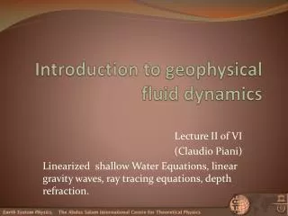
Introduction to geophysical fluid dynamics. Lecture I of VI ( C laudio Piani ) Course philosophy , the Navier -Stokes equations, Shallow Water, pressure gradient force, material derivative, continuity, linearization. 2. Course Philosophy .

E N D
Introduction to geophysical fluid dynamics Lecture I of VI (Claudio Piani) Course philosophy, the Navier-Stokes equations, Shallow Water, pressure gradient force, material derivative, continuity, linearization.
2 Course Philosophy • Start with a non stratified, incompressible, non-rotating , inviscid fluid (shallow swimming pool), and look at what happens away from the boundaries : • When the fluid is at rest • Immediately after the fluid is perturbed. • At equilibrium or steady state, long after the fluid is perturbed • Add elements of complexity one-by-one. • Rotation • Compressibility • stratification • Viscosity • Boundary effects • Geometry (spherical earth)
3 The simple case: shallow pool • The state of our shallow pool is completely determined by 3 variables: • h: the height of the free surface • u: the x-component of velocity • v: the y-component of velocity h v u
4 shallow pool: equations of motion Momentum equations Material derivative Mass continuity We have 3 independent variables (u,v,h), hence we require 3 equations to describe the evolution of the system. These are the 2 components of the momentum equation and the continuity equation. or Where: is referred to as the material derivative.
5 Material derivative The material derivative expresses the rate of change or a variable following the fluid parcel. It is a straight forward derivation of the rules of Total Differentiation: Dividing through by dt and remembering that da is the change of a following the fluid parcel motion, hence:
6 Material derivative Finally: Or in vector notation: Where: Is the fluid velocity.
7 Height (or pressure) gradient term The right hand side (RHS) of the momentum equations is the gradient of the height of the free surface h. It is easy to show that this is related to the pressure gradient. The pressure at point x+dx is equal to the pressure at x plus the added term due to the extra weight of the overlying fluid: This is true only because r is a constant Hence:
8 Pressure term You should already have derived this in previous classes. However should you be wondering how you got to the pressure term, here is a reminder: The x-acceleration imparted to the parcel of fluid parcel between x and x+dx is proportional to the force acting on the parcel at the x boundary (in the x direction) minus the force acting at the x-dxboubdary (in the –x direction).
9 Mass continuity The rate of change of mass in a unit area of the pool is equal the rate of change of the height of the fluid:
10 Mass continuity II Mass conservation implies that the rate of change of mass in a unit area of the pool is equal to the negative divergence (convergence) of flux of mass into that area (we will only do the one dimensional problem):
11 Mass continuity III If we move the advective term to the LHS and use the material derivative, we obtain:
12 Review: Shallow Water Equations (SWE)
13 SWE: linearization Even for this very simple physical model there are no analytic solutions. One way to circumvent the problem is to consider only small perturbations from a idealized simple steady state. This is a Powerful technique which you will adopt frequently in GFD. It is also referred to as linearization. We assume that the dynamical variables (h,u,v) that determine our system can be decoupled into two fields (h,u,v)=(h’+H,u’+U,v’+V) such that (H,U,V) are of very simple form. Also the perturbation quantities must be very small in the sense that:
14 SWE: linearization For example let’s consider the simplest possible case of a fluid of constant mean depth H where the background velocities zero. The SWE become: From which we can eliminate all the terms which are second order in the perturbation variables.
15 LSWE We obtain the linearized shallow water equations (LSWE) with no background motion.
16 EXERCISES: Consider the LSWE (slide 15). What is the only steady state solution possible for h? (Hint: steady state means: ) Derive the continuity equations in pages 10-11 for the 2 dimensional case. (hint: the equation on page 10 is unchanged. Take the 1st equation on page 11 and add the term for vh.)