Download
1 / 59
590 likes | 605 Vues
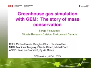
Greenhouse gas simulation with GEM: The story of mass conservation. Saroja Polavarapu Climate Research Division, Environment Canada. CRD: Michael Neish, Douglas Chan, Shuzhan Ren MRD: Monique Tanguay, Claude Girard, Michel Roch AQRD: Jean de Grandpré, Sylvie Gravel. RPN seminar, 6 Feb. 2015.

E N D
Greenhouse gas simulation with GEM: The story of mass conservation Saroja Polavarapu Climate Research Division, Environment Canada CRD: Michael Neish, Douglas Chan, Shuzhan Ren MRD: Monique Tanguay, Claude Girard, Michel Roch AQRD: Jean de Grandpré, Sylvie Gravel RPN seminar, 6 Feb. 2015
OUTLINE • What are we trying to do and why? • The mass conservation story of GEM for CO2 • Ensemble Kalman Filtering
Pg C/yr 8.6 The Global Carbon Cycle http://www.scidacreview.org/0703/html/biopilot.html 1 Pg = 1 Gt = 1015 g • The natural carbon cycle involves CO2 exchange between the terrestrial biosphere, oceans/lakes and the atmosphere. • Fossil fuel combustion and anthropogenic land use are additional sources of CO2 to the atmosphere. Net surface to atmosphere flux for biosphere or ocean is a small difference between two very large numbers Earth’s crust 100,000
Net perturbations to global carbon budget LeQuere et al. (2013, ESSDD) • Based on 2002-2012 • 50% of emissions remain in atmosphere • 25% is taken up by terrestrial biosphere • 25% is taken up by oceans
Interannual variability http://www.carboscope.eu/?q=co2_budget 25% uptake by land 50% to atmosphere 25% uptake by ocean • The uncertainty and interannual variability in the global CO2 uptake is mainly attributed to the terrestrial biosphere • Thus, we must first learn more about biospheric sources/sinks
But what is the spatial distribution of the fluxes and how is it changing? Mean XCO2 Aug. 2009 GOSAT Greenhouse Gas Observing Satellite v2.0 averaged at 0.9°x0.9° Figure courtesy of Ray Nassar, CCMR Figure courtesy of Elton Chan, CCMR With the increased coverage from new satellite data, can we get flux estimates at higher spatial resolution? OCO-2 launch July 2014 http://oco.jpl.nasa.gov/
Atmospheric observations give feedback on model forecasts • If forecast does not match observation, difference could be due to errors in CO2 initial conditions, meteorological analyses, prescribed fluxes, model formulation, representativeness, or observation errors. CO2 forecast Model error Forecast model Fluxes CO2 analysis Meteorology analysis
The inverse problem for Carbon Flux estimation • In flux inversions, if one solves for fluxes only, the transport model is needed to relate the flux to the observation: model is a strong constraint • Exact mass conservation in transport model over years of simulation is needed to attribute model-data mismatch to fluxes. • Techniques used to solve inverse problem: 4D-Var, EnsKF, Bayesian Inversion, Markov Chain Monte Carlo (MCMC) • Perfect model assumption since forecast model is used as a strong constraint • No allowance for imperfect meteorological analyses • Extension for imperfect tracer initial conditions is not hard flux Prior flux conc obs Forecast model Spatial interpolation
Conventional inverse problem setup 22 TransCom regions World Data Centre for Greenhouse Gases (WDCGG) http://transcom.project.asu.edu http://gaw.kishou.go.jp/cgi-bin/wdcgg/map_search.cgi Weekly avg obs Monthly mean flux J F M A M J J A S O N D J F M A M J J One or more years
Inversions using surface network Peylin et al. (2013) • Inversion methods differ in: • Methodology • Observations • Sfc: 100 flask + continuous • A priori fluxes • Transport models • Interannual variability is similar and due to land 1 5-6 27-8 39 410 11
The changing observing system Mean XCO2 Aug. 2009 GOSAT Greenhouse Gas Observing Satellite World Data Centre for Greenhouse Gases v2.0 averaged at 0.9°x0.9° http://gaw.kishou.go.jp/cgi-bin/wdcgg/map_search.cgi GOSAT figure courtesy of Ray Nassar, EC • ~100 highly accurate surface stations with weekly or hourly data • Regular aircraft obs over Pacific • Satellites: GOSAT (2009), OCO-2 (2014) +…
Environment Canada Carbon Assimilation System (EC-CAS) • An advanced, state-of-the-art assimilation system which will use ensemble forecasts to directly simulate various sources of model error. Comparable to systems in development for Japan, US, etc. • Will be run routinely but behind real time since it takes time for flux to reach measurement locations • Forward model: global operational air quality model 0.9° x 0.9° • Statistical method: Ensemble Kalman Smoother (ext. of oper.) • Observations: GAW global surface-based in-situ and remote sensing stations, satellite, aircraft, Total Carbon Column Observing Network (TCCON) • Emissions: biosphere (Canadian Terrestrial Ecosystem Model from CCCma), ocean, fossil fuel, biomass burning 13
Analysis step forecast step EC-CAS Carbon Assimilation System Flask, continuous, aircraft, satellite Perturb initial conc., met fields, fluxes Perturb obs
The future vision: Comprehensive Carbon Data Assimilation System Comprehensive carbon assimilation systems are being built by NASA, NOAA, agency-consortiums in Europe, Japan and EC. GEO Carbon Strategy Report (2010)
Saroja Polavarapu: (lead) data assimilation Mike Neish: system development Ray Nassar: satellite observations, modeling anthropogenic and other emissions Douglas Chan: carbon cycle science and modeling Bakr Badawy: biospheric modeling University collaborators: Prof. Dylan Jones (U Toronto), Feng Deng Prof. John Lin (U Waterloo), Myung Kim (U Waterloo) EC-CAS team
Global mean surface pressure 0-day forecasts Pressure (hPa) 10-day forecasts Date Operational model forecasts • 10-day forecasts from the current operational model (experimentK4H1RA2B: Strato2B final cycle) also show a steady drop in global mean surface pressure • About 0.1 hPa is lost in 10 days
Why do we need mass conservation? • When we assimilate greenhouse gas observations, mass conservation will not be possible. So no need for this if we want to estimate the CO2 or CH4 state only. • However, we need mass conservation for • Accurate forward simulations of CO2/CH4. With a good initial state and good source/sink inputs, can match observations. • Estimation of sources/sinks of CO2/CH4 with inverse methods. Such methods will serve as a benchmark for the non-traditional EnKF state/flux estimation scheme.
Greenhouse gas simulation with GEM-MACH • Need good simulation of GHG with exact mass conservation • Priorities: (1) CO2 global (2) CH4 global (3) CO2, CH4 regional • CH4 chemistry: (D.Chan, CCMR) • stratosphere – LINOZ (de Grandpré, McLinden, AQRD), • troposphere: • [OH] climatology from CMAM (D. Plummer, CCCma) • Start with global CO2 simulation Physics emis+v.diff Dynamics Dynamics Physics emis+v.diff MACH MACH RPN RPN GEM GEM
Model validation: experiment setup How well can GEM-MACH simulate Carbon? Simulation for January 1 – December 31, 2009 Initial condition from CarbonTracker for Jan. 1, 2009 Meteorology: surface fields (archived surface analyses), 3D winds, archived analyses from 4D-Var Set up: series of 24h forecasts, no CO2 assimilation Emissions: Every 3 hours (area type) though GEM-MACH set up for monthly fields with diurnal variation biosphere (CarbonTracker a posteriori) ocean (CarbonTracker a posteriori) Fossil Fuel (CarbonTracker but based on CDIAC) Biomass burning (GFED v3) Idea: With CarbonTracker emissions and initial conditions, simulation should match CarbonTracker if transport is similar
Lack of global mass conservation • Because of emissions, large gradients near the surface are created. The semi-Lagrangian advection scheme does not conserve mass. • The poor vertical mixing of CO2 from the surface exacerbates the non-conservation issues. 10 20 50 Increasing KTmin reduces increase in global CO2 Petagrams C Time
Hypothesis • Hypothesis: Adding fluxes at the surface creates large horizontal gradients. Without sufficient vertical mixing in the boundary layer, these unrealistically large gradients are smoothed by the semi-Lagrangian advection scheme (nonconservative flavour). With fast vertical mixing, horizontal gradients are reduced before the SL scheme can act. • To prove this: Check global mass before and after advection and before and after diffusion • Mass change due to diffusion is machine precision • Mass changes due to advection!
Further proof: Turn off advection control 4.5 Pg C = 2.1 ppm too much Annual growth is 7.7 Pg but should be ~4 Petagrams C No advection Time
How did we accumulate so much CO2? Mass change due to advection over 24 h • The mass change due to advection over 24h is shown • 7.7 Pg C per year is 0.0004 Pg C per time step for monotonic changes. • For global CO2 of 818 Pg C only 0.00006 Pg C can be represented with 32-bits. • The error we are looking for is only 6.7 times machine epsilon Mass change (Pg C) 0.028 Pg C Hour
Mass conservation: Semi-Lagrangian advection Houweling et al. (2010, ACP) • ECMWF IFS (red) shows spurious increase of 1 ppm (Recall GEM spurious increase of 2.1 ppm in one year) • South Pole (or Darwin) shows background CO2 values best and better illustrates annual trend Simulated and observed XCO2 1 ppm IFS LMDZ TM3 TM5 obs Pg C
EC-CAS version: GEM v4.6.0-rc8 • Factors found to reduce spurious mass gain: • Reducing time step • Adding horizontal diffusion to tracers consistent with meteorological fields • Including convective transport of tracers (Zhang-McFarlane scheme) • Adding tracer mass conservation scheme with global mass fixer (Bermejo-Conde) Without tracer mass conservation scheme With Bermejo-Conde+ILMC scheme Petagrams C After one year, difference in mass from expected mass is 0.04 Pg C Mismatch in summer when global water vapour cycle peaks Time
Global mass of water vapour in GEM analyses during 2009 The total mass of the atmosphere varies mainly due to water vapour loading. • Trenberth and Smith (2005, J.Clim.) • The mass of dry air is constant • Water vapour cycle amplitude is 0.36 hPa or 0.00037 rel. to dry air • Here amplitude is 1900/5E6=0.00038 Petagrams Time
Next puzzle • Why don’t we get exact mass conservation even after we (Monique Tanguay) implemented a tracer mass conservation scheme? • Tracer variable in model • Presently a pseudo moist mixing ratio (mass CO2/mass moist air). (Mixing ratio is NOT adjusted whenever water vapour changes, e.g. after physics step.) • Tracer mixing ratios defined w.r.t. dry air is another way • Observations are of mixing ratio w.r.t. dry air (mass CO2/mass dry air) • Let’s check global mass of CO2, air and water vapour at various points in the model time step.
Terminology used here Dynamics Dynamics Emis+diffus Emis+diffus Physics Physics Adv+? Adv+? “Advection” change “Diffusion” error “Advection” change “Diffusion” error Mass change due to “advection” actually includes any changes anywhere in the dynamics or physics steps.
GEM does not conserve global moist air mass without use of switch PSADJ Global moist air mass • About 2500 Pg of moist air is lost in 10 days. • This is a relative loss of 0.0005 PSADJ=on PSADJ scheme PSADJ=off Petagrams Day in January 2009
Impact of switch PSADJ Mass change due to dynamics+physics steps • Turning PSADJ on removed the H2O signal from moist air mass 2 0 -2 -4 -6 -8 -10 10 5 0 -5 -10 -15 -20 PSADJ=on PSADJ=off PSADJ=on PSADJ=off PSADJ seems to remove water! Air mass include H2O signal Petagrams Ideally red curve should look like this Water vapour Moist air 1 3 5 7 9 1 3 5 7 9 January 2009 January 2009
A missing source of mass for Ps • Claude Girard (RPN-A) determined that the changes in global water vapour due to physics impact GEM’s thermodynamic equation but the flux of water across the Earth’s surface was not properly accounted for. • We need to use the surface pressure to compute the total air mass and we assume that the water vapour mass is accounted for when computing tracer mass. If the surface pressure does not reflect the current mass of water vapour, global tracer mass calculations will not be accurate. • Claude devised a means of adding this source of mass to surface pressure at the end of the physics time step (see his Note from August 19, 2014). http://iweb.cmc.ec.gc.ca/~armasmp/docs/mass-cons/Total_mass_variation_iin_GEM_girard.pdf • Monique Tanguay (RPN-A) implemented this in GEM v4.7.0 and v4.6.0-rc8
Impact of new mass source of Ps Mass change due to dynamics+physics steps • With adw_source_ps=True, moist air mass change from one time step to the next resembles water vapour mass change, as hoped Adw_source_ps=True Adw_source_ps=False Moist air Water vapour Hours from May 1, 2009 0UTC Hours from May 1, 2009 0UTC
Impact of ps_source on air mass Air mass evolution over 10 days • PSADJ acts on moist air • We actually need PSADJ to act on dry air PS_source on PS_source off PS_source on PS_source off Petagrams Moist air mass Dry air mass Hours from Jan. 1, 2009 00Z Hours from Jan. 1, 2009 00Z
New ps_source term will impact meteorological forecasts Expt by Monique Tanguay 2 day forecast valid 3 Jan 2009 Difference in surface pressure due to new Ps mass source • Differences are largest in the tropics and in synoptic scale systems over the ocean • Max differences are about 3 hPa! • There may be an impact on meteo forecasts
Forecast impact of ps_source: NH summer/winter (neg/neutral) Expts by Michel Roch GYY15 96h SH NH Tropic Control Ps_source u u u u u u uv uv uv uv uv uv Summer GZ GZ GZ GZ GZ GZ T T T T T T Winter
Another new flag: PSADJ-dry • For both experiments: PS_source is on • Good conservation in first 24 hours PSADJ on moist air PSADJ on dry air Spurious increase in dry air mass 10 day change is 100/5.1E6=2E-5 Petagrams 10 day change is 10/5.1E6=2E-6 Better but not perfect conservation of dry air Dry air mass Hours from Jan. 1, 2009 00Z
Impact of ps_dry: Neutral Expts by Michel Roch GYY15 96h SH NH Tropic u u u u u u uv uv uv uv uv uv Summer GZ GZ GZ GZ GZ GZ T T T T T T Winter
Need a dry mixing ratio for tracers Change in CO2 mass • No tracer mass conservation. Keep PSADJ-dry=on, PS_source=on. • Define CO2 mixing ratio as 𝜒=𝜌CO2/𝜌dry-air instead of 𝜒=𝜌CO2/𝜌air • Dry mixing ratio removes water signal, and CO2 is more constant but still need to add tracer mass conservation scheme for this variable. • This was done by Monique Tanguay CO2 mixing ratio w.r.t. moist air CO2 mixing ratio w.r.t. dry air • Spin-up problem • CO2 change is ~0.0001 Pg C • Diffusion error is <0.0000005 PgC Petagrams Hours from Jan. 1, 2009 00Z
CO2 global mass with a dry tracer mixing ratio Dry tracer mixing ratio • With a tracer mixing ratio w.r.t. dry air, mass conservation is good until October then drifts • Accounting for local changes in air mass (surface pressure) when analyses are inserted every 24h yields exact conservation! But CO2 fields are terrible—so the story is not over... Petagrams C Local offset scheme Dry tracer mixing ratio normalized Expected mass Time
Good agreement with surface obs Dry tracer mixing ratio, global offset scheme Without assimilation, CT fluxes Obs GEM Alert Sable Island Toronto
CO2 transport with GEM compared to chemistry transport models Column mean CO2 for 2009 The model runs use the same initial state and fluxes GEM GEOS-CHEM (US academia) CarbonTracker (NOAA)
Relevance of greenhouse gas modeling work to GEM • Feedback to GEM-MACH: • https://wiki.cmc.ec.gc.ca/wiki/EC-CAS_Technology_Transfer • Vertical diffusion equation • Emissions coding error • Assessing vertical diffusion equation in dry mixing ratio • Feedback to GEM • Helping to test tracer conservation schemes • Illustrated a missing source of mass for surface pressure • Involved in redesign of global mean surface pressure fix • Helping to convert tracer equation to dry mixing ratio Dynamics Dynamics emis+v.diff Physics emis+v.diff Physics MACH MACH RPN RPN GEM GEM
Ensemble Kalman Filter – first look • No tracer assimilation, only passive advection • Testing with 64 ensemble members, 0.9° grid spacing • Start on 28 Dec 2008. Run for 4 weeks to 23 Jan 2009 • All members have same initial CO2 and same fluxes. Spread is due to spread in winds only. • Winds differ among ensemble members due to differences in: model parameters (convection scheme, parameters involved in PBL model, diffusion of potential temperature, etc. ), observation error perturbations • How does uncertainty in winds affect CO2 spread?
Evolution of ensemble spread Animation of column mean CO2 Dec. 28, 2008 to Jan. 23, 2009 Ensemble mean Ensemble spread
Other coupled meteorology/tracer forecast systems • ECMWF: Real time operational 5-day CO2 forecasts since 2013. No assimilation of CO2 obs. Updated initial conditions from flux inversions every Jan. 1. Plans: Near-real time assimilation of surface obs of CO2 with coupled meteorological/tracer assimilation • NASA/Goddard GEOS5: Coupled CO and CO2 assimilation to meteorological assimilation. Weakly couple ocean and land data assimilation systems to atmospheric assimilation system. • Provide boundary conditions for regional modelling and flux inversions. • Improve modelling of radiative transfer, evapotranspiration • Feedback on modeling of boundary layer, convection, advection • Provide a prioris for satellite retrievals of CO2 and CH4
Future work • EnKF development (Polavarapu/Neish) • compare to obs without CO2 assimilation • Extend EnKF for tracer assimilation • Global methane simulations (D.Chan) • Tropospheric chemistry uses CMAM OH climatology (D.Plummer) • Stratospheric chemistry from Jean deGrandpré (LINOZ) • OCO-2 OSSE work (Ray Nassar) • Regional greenhouse gas simulations to support inverted Lagrangian trajectory work • supports measurement network interpretation work of Elton Chan and Douglas Chan • Coupling with CTEM (CCCma ecosystem model) (Bakr Badawy) • Evaluate CTEM with GEM meteorology