Understanding Local and Global Optima in Linear Programming
This lecture delves into the essentials of linear programming (LP), focusing on the relationship between local and global optima. Key definitions are provided, explaining that every local optimum is a global optimum and that extreme points in a convex set hold unique significance. Examples illustrate situations where LPs can possess interior points as optimal solutions. The session also covers how to convert standard notations and handle inequalities in LP formulation, ensuring a comprehensive understanding of solving linear programming problems through algebraic methods.

Understanding Local and Global Optima in Linear Programming
E N D
Presentation Transcript
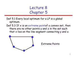
Lecture 8Chapter 5 • Def 5.1 Every local optimum for a LP is a global optimum. • Def 5.3 If x is an extreme pointof a convex set, then there are no other points y and z in the set such that x lies on the line segment connecting y and z. Extreme Points
Unique LP Optimum • Def 5.5 If an LP has an optimum, then it has some extreme point that is an optimum. • (There may be other points that are optimal as well.) Unique Optimal Solution
Infinite Number Of Optimal Solutions • Infinite number of optimal solutions. Do we have an extreme point that is an optimum?
Interior Point That Is An Optimum • Please give an example of a LP that has an interior point as an optimum. Minimize cx What is c, so that red point is an optimum?
Standard Notation For LPs • Minimize j cjxj • Subject to • j aijxj = bi, all i • xj> 0, for all j • Minimixe cx • Subject to • Ax = b • x > 0 Summation Notation Matrix Notation
Converting To Standard Notation • Converting inequalities to equalities • 2x + y < 10, x > 0, y > 0 • Becomes • 2x + y + s = 10, x > 0, y > 0, s > 0 • Try it • x = 3, y = 3.5 • Implies that s must be 0.5 • How do you handle 2x + y > 10, x > 0, y > 0
Solving Systems Of Equations • (Finding The Inverse By Inspection) • Example #1 • X1 + X2 = 10 • -X1 = -5 • -X2 – X3 = -3 • In matrix notation we have Bx = b b = B =
B-1 Is Inverse Of B • BB-1 = I = • Find B-1 by inspection
Matrix Multiply • B B-1 = I • Matrix Multiply: Row r of B time Col c of B-1 • Produces the r,c element of the result
Determine 1st Row • B B-1 = I • Matrix Multiply: Row r of B time Col c of B-1 • Produces the r,c element of the result
Determine 2nd Row • B B-1 = I • Matrix Multiply: Row r of B time Col c of B-1 • Produces the r,c element of the result
Determine 3rd Row • B B-1 = I • Matrix Multiply: Row r of B time Col c of B-1 • Produces the r,c element of the result
Solution To Equations • x = B-1b = = • Check The Solution X1 = 5, X2 = 5, X3 = -2 • X1 + X2 = 10 • -X1 = -5 • -X2 – X3 = -3
Example 2 • X1 + X2 = 10 • -X1 = -2 • X3 = -3 • X4 = -1 • -X2 – X3 – X4 + X5 = 2 • Bx = b
What Row Do We Find First? • B B-1 = I
Row 3 • B B-1 = I
Row 1 • B B-1 = I
Row 2 • B B-1 = I
Row 4 • B B-1 = I
Row 5 • B B-1 = I
Solution • Solution is given by x = B-1b =
Check • X1 = 2, X2 = 8, X3 = -3, X4 = -1, X5 = 6 X1 + X2 = 10 -X1 = -2 X3 = -3 X4 = -1 -X2 – X3 – X4 + X5 = 2
To Solve LPs • To solve linear programs, we have to solve a sequence of systems of equations. Actually, we solve • vB = cB and By = aj • for v any y at each iteration (step). • cB, B, and aj are all original data in the problem.