Download
1 / 55
550 likes | 754 Vues
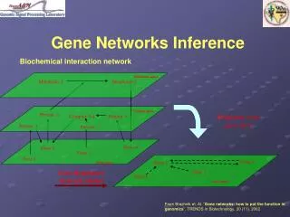
Metabolic space. Metabolite 1. Metabolite 2. Protein space. Protein 2. Complex 3-4. Protein 4. Protein 1. Protein 3. Gene 4. Gene 2. Gene 3. Gene 1. Gene space. Gene Networks Inference. Biochemical interaction network. Projection to the gene space. Gene 4. Gene 2.

E N D
Metabolic space Metabolite 1 Metabolite 2 Protein space Protein 2 Complex 3-4 Protein 4 Protein 1 Protein 3 Gene 4 Gene 2 Gene 3 Gene 1 Gene space Gene Networks Inference Biochemical interaction network Projection to the gene space Gene 4 Gene 2 Gene Regulatory Network Model Gene 3 Gene 1 Gene space From Brazhnik et. Al. “Gene networks: how to put the function in genomics”, TRENDS in Biotechnology, 20 (11), 2002
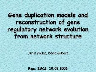
Example: kinetic equations Rate = src RNAP degradation U RNAnuc mRNAnuc Gene G Amino acids Transcription factor RNAcyt mRNAcyt Enzymatic reaction P AA Source material Translated product of the mRNA. It goes to the nucleolus to repress the gene G, but it is subject to degradation, so eventually G can be reactivated Rate = From Hucka et. Al. “The system biology markup language (SMBL): a medium for representation and exchange of biochemical network models”, Bioinformatics, 19 (4), 2003
Considerations • Too many parameters: Vi, Km3, .... • To know the model, we need to know the parameters that define it • Needs lots of data to estimate the parameters • Solution: simplification of the model U Transcription factor Gene G
Example of Cell Cycle Regulation Logic diagram AND gate outputs cdk2; p21/WAF1 is the input for a NOT gate; NAND gate outputs Rb
Predictive Relationships * • To discover predictive relationships, we let each gene be the target and design filters for each combination of one, two, three, and four predictor genes. • Coefficient of Determination (COD) : * Kim et. al., J. Biomedical Optics, 5(4), Oct 2000.
Boolean Formalism * • Studies give rise to qualitative phenomena, as observed by experimentalists. • Studied systems exhibit multiple steady states and “switch like” transitions between them. • For practical approximation, gene regulatory networks have been treated with a Boolean formalism (i.e. ON/OFF). * Stuart A. Kaufman, Origin of Order : ‘Self-Organization and Selection in Evolution’, Oxford Univ. Press, 1993
Gene G1 Gene G2 Gene G3 Gene G4 Bottom-Up approach: Boolean functions • Assume Gene G4 is biologically “regulated” by Genes G1 ,G2 and G3 • If we find this relationship (rules), we can combine them to have a full-network information • Goal: to find the genes that “regulate” G4
Important • The Boolean function model is for the biological model, NOT for the observed data !!! • Each binary function mimics the biological behavior with some degree of fitness. • The quality of this fitness can be measured via an error measure • There is always an optimal binary function, that best fits the biological model.
Model: Boolean functions • Activity of gene 1 (promoter) promotes the activation of gene 3, unless gene 2 is active (repressor). Gene 1 f3 Gene 2 Gene 3 A possible Boolean function to represent this biological relationship
Inference of Boolean Functions Boolean relationship between genes can be estimated from microarray data. Experiment 1 Experiment 2 Experiment 3 Experiment 4 Experiment 5 Experiment 6 Experiment 1 Experiment 2 Experiment 3 Experiment 4 Experiment 5 Experiment 6 Examples: A B C Experiment 1 0 0 1 Experiment 2 0 1 0 Experiment 3 1 1 0 Experiment 4 1 1 1 Experiment 5 1 1 1 Experiment 6 0 0 1 Gene A Gene A 0 0 1 1 1 0 Gene B Gene B 0 1 1 1 1 0 Gene C Gene C 1 0 0 1 1 1 Gene D Gene D 1 0 0 0 1 1 A B Boolean function fc for C A B C 0 0 1 0 1 0 1 0 X 1 1 1 fC C
Connectivity of BN • Predictor set for BN: W := (W1,…, Wn) • Minimum predictor set ~ BN Connectivity • Compatibility between W and the state transition diagram • BN Connectivity and its relation to the regime of functioning: ordered, chaotic or on the edge of chaos
State Transition Diagram 100 100 100 100 100 100 100 100 100
Interpretation of the State Transition Diagrams • Attractors/fixed points ~ cellular types or cellular states, such as proliferation, apoptosis, and differentiation • Basins of attraction ~ structural stability or ordered collective behavior * Stuart A. Kaufman, Origin of Order : ‘Self-Organization and Selection in Evolution’, Oxford Univ. Press, 1993
Problem: to find the connection between genes Gene 4 Gene 2 Gene 3 Gene 5 Gene 1 Gene space CoD Gene 1 Gene 2 Gene 3 Gene 4 Gene 5 Gene 1 Gene 2 Gene 3 Gene 4 Gene 5
Error measure for binary functions • How good is this function to “model” the relationship between G1,G2 and G3 ? • The quality of the function depends on the “joint” distribution of G1,G2 and G3 • In the same way, if the constant function is defined by 0=c
G1 G2 G3 Boolean Functions • If the expression of the genes is assumed to have 2 possible values (0 – inactive,1 - active), we can use Boolean functions to “model” the relationship between the genes. One example of a Boolean function All possible combination of values for the pair {G1,G2}
G1 G2 G3 Constant Functions • The behavior of the gene G3 can also be predicted by a constant function. • In this case G3 doesn’t depend on G1 and G2, so we can write “ = 0 = c ” to specify the function (The sub-index 0 in 0 denotes the absence of predictors) Example of a constant function
Optimal Function • Between all possible Boolean functions , one of them has the minimal error, as predictor of G3 from G1 and G2. This function is called opt. • [opt] [] for any other Boolean function • If G1 and G2 are good predictors of G3, then the relationship between them will be “captured” by optand [opt] will be small. • The optimal constant predictor is called 0-opt. (there are only 2 possible constant predictors: 0 and 1). • If G3 is almost constant, then [0-opt] will be small.
Coefficient of Determination • The Coefficient of Determination (CoD) of the pair of genes G1 and G2 as predictors of the gene G3 is given by the relative improvement in the prediction when using the optimal predictor optover the optimal constant predictor 0-opt. • The CoD depends ONLY on the joint distribution of G1,G2 and G3.
Estimation of the CoD for G1,G2 and G3. Microarrays Example of a Binary Expression Matrix Estimation of the optimal functions optand 0-optfor {G1,G2} as predictors of G3 Estimated CoD for {G1,G2} as predictors of G3
Estimation of [opt] for G1,G2 and G3 from the data Ternary Expression Matrix for G1,G2 and G3 Splitting of the matrix in Training and Test sets
Estimation of [opt] for G1,G2 and G3 from the data More frequent value computed from data (X denotes a non- observed configuration) Generalization to fill non-observed configurations Statistical Inference of the optimal function opt. Estimation of the error of [opt] from test set 1 mistake on 4 *[opt]= 0.25
Estimation of [0-opt] for G1,G2 and G3 from the data Frequencies of possible values of G3 on train data Statistical Inference of the optimal function 0-opt. 0-opt. = 1(use heuristic) (most frequently observed value for G3) Estimation of the error of [opt] from test set 3 mistakes on 4 *[0-opt]= 0.75
Estimation of the CoD for G1,G2 and G3 from the data *[opt]= 0.25 *[0-opt]= 0.75 The error is reduced in a 66 %
Estimation of the CoD for G1,G2 and G3. • The previous process is repeated 1000 times, with different random splitting of the set in training and test sets. • The estimated value for the CoD is the average of the 1000 values of *. • If we want to know the predictive power of other pair of genes, say G4,G5, over G3, we must repeat the whole process • G1,G2 G3 312 • G4,G5 G3 345
Methodology • Compute the CoD for all sets of 1,2 and 3 predictors for each target gene. 1 predictor 2 predictors 3 predictors Gene 2 Gene 2 & 3 Gene 3 & 4 Gene 2,3,4 Gene 3 Gene 2 & 4 Gene 3 & 5 Gene 2,3,5 Gene 4 Gene 2 & 5 Gene 4 & 5 Gene 2,4,5 Gene 5 Gene 3,4,5 Gene 1 Quality of prediction : CoD
Results • Most probable predictors sets for each gene Gene 2 Gene 2 e 3 Gene 2,3,4 Gene 1 2 23 234
Gene 1 Gene 2 Gene 3 Gene 4 Gene 5 Gene 1 Gene 2 Gene 3 Gene 4 Gene 5 Results • Determination of the predictive genetic network
Discussion • The CoD can be applied to ternary data, more general discrete data and on continuous data, restricting the family of functions (linear, neural network, etc) • This technique is a “feature selection” technique analyzing all the possibilities. Existing algorithms can be applied to optimize the search, in detriment of the quality of the result (ex: genetic algorithm, sub-optimal search)
Conclusions about CoD • CoD is a useful tool in the determination of the predictive genetic network • Computationally expensive: feasible only for 3 predictor sets for moderate sets 200-500 genes • Does not give information about the functions, but they can be estimated easily from the data
Regulatory diagram for the activation of the tumor-suppressor protein p53 Vogelstein, B., Lane, D. &Levine, A. Surfing the p53 network. Nature 408, 307-310 (2000)
Probabilistic Boolean Networks • Share the appealing rule-based properties of Boolean networks. • Allows to model randomness • Explicitly represent probabilistic relationships between genes. • Robust in the face of uncertainty. • Dynamic behavior can be studied in the context of Markov Chains. • Boolean networks are just special cases. • Allows quantification of influence of genes on other genes.
PBN PBN := ({BN1, …, BNk}, p1, …, pk, p, q) 0 < p < 1 - probability of switching context 0 < pi < 1 – probability for BNi being used 0 < q < 1 – probability of gene flipping Context := Which BN is used for the next transition ~ the regime in which the cell operates/functions Gene flipping ~ mutation rate
Probabilistic Boolean Networks vs. Boolean Networks x1 x2 x3 xn Boolean Networks xi x1 x2 x3 xn Probabilistic Boolean Networks xi
p1 q p2 p
Context Switching X2 X2 X3 X3 p X1 X1 p1 q p2
PBN • Different combination of functions determines different Boolean Networks • The model can be seen as a Markov Chain, where the transition is deterministic once decided (randomly) which Boolean Network to use • Properties of the Boolean Networks determine properties of the Markov Chain • Transition probabilities • Stationary distributions • Steady-states (long run behavior) • (We are not so interested in transients)
Probabilistic Boolean Networks • Influence : determinative power of the variables (genes) • Intervention : changing the behavior of some genes to make the network to transition to desired states • External control : PBNs depending on external (control) variable. Interest in treatment strategies
Attractors in PBNs Attractors in the Boolean Networks should correspond to cellular types (Kauffman) • PBNs are formed by a family of Boolean Networks • Steady-state analysis of the PBN may be meaningful for classification based on gene-expression data • Relationships between steady-state distribution and the attractors of the Boolean Networks allow for structural analysis of the network
Dynamics of PBNs with perturbations The same Boolean Network being used Time In a basin In the Attractor Change of function or perturbation The system reaches the Attractor Next change of function or perturbation
Steady-state analysis • Steady-state: The state probability distribution of the network in a long run • In the long run, the system is expected to stay in the attractors of the Boolean Networks From the same initial point the system can transition to two different regions (attractors) depending on the Boolean Function being used
BN with perturbation • A state of the BNp is a vector s=[x1,…,xn] є {0,1}n • p є (0,1]: models random gene mutations: • At each time point, there is a probability p for any gene to change its value uniformly randomly, therefore: • Markov Chain is ergodic and aperiodic Steady- State Distribution (SSD) exists
Control Policy • A control policy Πg = {µ(t)}t>0 based on gene g, is a sequence of decision rules µg(t) : S {0,1} at each step t, where: • S: collection of all states s of the network • 0/1: not flipping/flipping the control gene • MFPT control policy: • Stationary for each candidate gene
Mean First Passage Time(MFPT) Algorithm* • Intuition behind the algorithm: • Given the control gene g, if desirable state s reaches U on average faster than ŝg , it is reasonable to apply control and start the next network transition from ŝg • More formal display of the algorithm: • For all states s in U (ŝg flipped control gene in s) : • If KD(s) - KD(ŝg) > γ then • µg(s) = 1 • else • µg(s) = 0 • Considering therapeutic interventions, states can be divided into 2 sets: • D: Desirable • U: Undesirable • KU: a vector containing MFPTs from each state in D to U • KD: a vector containing MFPTs from each state in U to D • γ: tuning parameter • γ is set to higher value when “cost of the control/cost of undesirable state” is higher, for applying less control
Methodology • Inducing control policy of the reduced network to the original network • Genes that cannot be deleted: • MFPT control policy for the original network is designed and has 2n decision rules • MFPT control policy of the reduced network is designed and has 2n-1 decision rules, since the number of genes is n-1 in the reduced network • The control policy designed on the reduced network, induced to another control policy for the original network • The original and induced control polices of the original network were compared • Xi: partitions states into D and U • Xj: control gene
Simulations • 100 BN0.1 • n= number of genes = 7 • γ: tuning parameter in MFPT algorithm • γ has the range 0-6 with 200 equally spaced values • The same values of γ were used for designing control policies in original and reduced network • Hamming Distance is used for measuring the difference between the original MFTP CP and induced CP of the original network
Results – Inducing CP Average Hamming distance for 100 BN0.1, 200 different Gammas