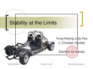
Stability at the Limits
Explore how loss of control in vehicles can be prevented by designing a control system that stabilizes nonlinear handling, communicates limits to drivers, and ensures consistent responses. Understand tire forces, nonlinear regions, and driver input saturation. Learn about tire parameter estimation, feedback linearization, and controller design. See how to track desired trajectories and manage driver input saturation to keep the vehicle safe. Discover how applying linear control theory leads to predictable vehicle behavior and reduces sideslip.

Stability at the Limits
E N D
Presentation Transcript
Stability at the Limits Yung-Hsiang Judy Hsu J. Christian Gerdes Stanford University November 10, 2005
did you know… • Every day in the US, 10 teenagers are killed in teen-driven vehicles in crashes1 • Loss of control accounts for 30% of these deaths • Inexperienced drivers make more driving errors, exceed speed limits & run off roads at higher rates • In 2002, motor vehicle traffic crashes were the leading cause of death for ages 3-33.2 To understand how loss of control occurs, need to know what determines vehicle motion 1 National Highway Traffic Safety Administration. Traffic safety facts (2002) 2 USA Today. Study of deadly crashes involving 16-19 year old drivers (2003) 2
motion of a vehicle SIDE VIEW • Motion of a vehicle is governed by tire forces • Tire forces result from deformation in contact patch • Lateral tire force is a function of tire slip Contact Patch Ground BOTTOM VIEW a Fy 3
tire curve maximum tire grip Linear Saturation Loss of control 4
vehicle response • Normally, we operate in linear region • Predictable vehicle response • But during slick road conditions, emergency maneuvers, or aggressive/performance driving • Enter nonlinear tire region • Response unanticipated by driver 5
loss of control Imagine making an aggressive turn • If front tires lose grip first, plow out of turn (limit understeer) • may go into oscillatory response • driver loses ability to influence vehicle motion • If rear tires saturate, rear end kicks out (limit oversteer) • may go into a unstable spin • driver loses control • Both can result in loss of control 6
overall goals We’d like to design a control system to • Stabilize vehicle in nonlinear handling region • Make vehicle response consistent and predictable for drivers • Communicate to driver when limits of handling are approaching 7
Outline • Identify tire operating region • Vehicle/Tire models • Tire parameter estimation • Produce stable, predictable response • Feedback linearizing controller • Driver input saturation • Simulation results 8
vehicle model Bicycle model • 2 states: β and r • Nonlinear tire model (Dugoff) • Steer-by-wire Assume • Small angles • Ux constant 9
equations of motion Sum forces and moments: Dugoff tire model: -C 10
tire estimation algorithm • Find f: use GPS/INS • Find Fyf: SBW motor give steering torque • Estimate C f and • LS fit to linear tire model • NLS fit to Dugoff model • Compare residual of fits to tell us if we’re in the nonlinear region estimate 11
parameter estimates • Begin estimating after entering NL region • C f estimate is steady 15
controller design • Desired vehicle response • Track response of bicycle model with linear tires • Be consistent with what driver expects • When tires saturate, compensate for decreasing forces with steer-by-wire input • One input f; two states ,r • Could compromise between the two • Or, track one state exactly 16
feedback linearization (FBL) • Nonlinear control technique Applicable to systems that look like: • Use input to cancel system nonlinearities. In our case, • Apply linear control theory to track desired trajectory: 17
FBL in action • Ramp steer from 0 to 4o at 20 m/s (45 mph) in 1 s • Controller results in exact tracking of linear tire model yaw rate trajectory 18
FBL in action • Ramp steer from 0 to 6o at 20 m/s (45 mph) in 1 s • FBL works well up to physical capabilities of tires 19
driver input saturation • Road naturally saturates driver’s steering capability often unexpectedly • Here, we safely limit steering capability in a predictable, safe manner • Why do we need it? • Prevents vehicle from needing more side force than is available • Keeps vehicle in linearizable handling region • Saturation algorithm • If < th, driver commands are OK • If ¸th, gradually saturate driver’s steering capability 20
overall control system • Ramp steer from 0 to 6° at 20 m/s (45 mph) in 1 s • Tracks linear model yaw rate, then saturates input • Reduced sideslip 21
design considerations • Relative importance of vs. r • Which produces a more predictable response? • Could add additional input to track and r • differential drive • rear steering 22
conclusions • Overall approach • Sense tire saturation and actively compensate for them with SBW inputs • Algorithm can characterize tires (C, ) using GPS-based f and estimates of Fyf, • Make vehicle response more predictable • Up to capabilities of tires, controller tracks linear yaw rate trajectory • Reduces sideslip • Current work • Estimate C, on board in real-time • Implement overall controller on research vehicle 23
controller validation • Simulate control system on more complete vehicle model 25
validation results II • input: ramp steer from 0 to 5° at 45 mph in 0.5 s 26
4 cases Case 1: Both tires are linear (f¸ 1 and r¸ 1) Case 2: Both tires saturating (f < 1 and r < 1) 27
4 cases Case 3: front is nonlinear, rear is linear (f¸ 1 and r < 1) Case 4: front is linear, rear is nonlinear (f¸ 1 and r < 1) 28
new inputs • Define new inputs v1 and v2 to represent system as 29
More general form of FBL SISO algorithm: 30
Front steering only approach • Model Fyf as: • Substitute into system equations: 32
Tracking yaw rate • Choose new input cr = 200 c = 50 33
Estimating Cf • Find f:Use GPS/INS to measure r and f and estimate • Find Fyf: Estimate tm from steering geometry, model tp as and use disturbance torque estimate from SBW system to find Fyf • Estimate : • Using least squares 34
Experimental Tire Curve • P1: Ramp steer from 0 to 9° in 24 s at V = 31 mph shad_2004-12-11_l.mat 35
questions? 36
overview • Motivation • Background • Controller design • Feedback linearization • Driver input saturation • Validation on complex model • Conclusions 37
steer-by-wire Removes mechanical linkage between steering wheel and road wheels • electronically actuate steering system separately from driver’s commands • decouple underlying dynamics from driver force feedback Conventional steering Steer-by-wire 38
comparing vehicle responses • Ramp steer to from 0 to 4o at 45 mph in 0.5 s 41
tire estimation algorithm • Find f: GPS/INS measures , r, V • Find Fyf: SBW motor give steering torque • Estimate C f and from (Fyf, f) data • LS fit to line • NLS fit to Dugoff Compare fit errors to tell us if in nonlinear region 42