Download

1 / 35
350 likes | 452 Vues
This document details the methodology and findings from assembling geophysical data to model the seismic response in Las Vegas Valley between May 2003 and May 2005. Key activities include the creation of shallow shear-velocity transects, extensive reconnaissance, and data integration to support LLNL. The study highlights significant correlations between seismic responses and subsurface characteristics, with insights on velocity variations and the implications for hazard mapping. The Model Assembler tool synthesizes existing geological data to improve seismic response modeling.

E N D
Assembling Geophysical Data to Model Seismic Response in Las Vegas Valley John G. Anderson & John N. Louie Seismological Lab, UNR May 2003 - May 2005
LVVSR Components @UNR • Shallow shear-velocity transects • Extensive reconnaissance data • Model Assembler • Enables LLNL to use existing knowledge • Adding new data; interoperation and archiving • E3D sensitivity studies • Place facilities and expertise at UNR • Guide model assembly
Shallow Shear-Velocity Transects • ReMi measures Rayleigh dispersion with linear refraction arrays.
Refraction Microtremor for Shallow Shear Velocity ReMi has classified hard and soft sites around the world by measuring V30, average shear velocity to 30 m depth.
Shallow Shear-Velocity Transect Las Vegas route from Cheyenne to Tropicana Supported by DOE-LLNL and IRIS-PASSCAL
Las Vegas Transect Some correlation to faulting, soil type?
Las Vegas Transect V100 echoes V30
850 m/s 3400 m/s Las Vegas Transect • Section to 200 m depth shows effects of faulting, high-velocity cemented layers. • How real are the rapid lateral variations?
Transect Data High-velocity picks at >0.4 sec period are unreliable. Picks at 0.1-0.3 sec illustrate velocity differences to 100 m depth.
Fit at 9.9 km Fit at 9.1 km Low confidence Whole array Deep layer misfit starts Deep layer starts not fitting <0.4 s Fitting Longer Periods
Las Vegas Transect No correlation between V30 and geologic map.
Las Vegas Transect Correlation with clay soils, caliche in Las Vegas?
A Preliminary Las Vegas Hazard Map Transect V30 values correlated with soil-map units across 4 quadrangles in Las Vegas Valley
ModelAssembler • A code to stitch together existing regional geophysical and geological data sets, into a form useful to E3D.
Model Assembler Operation Outline 1. Self-document and get infile name from command line Usage: java ModelAssembler file.in > file.out Run from UNIX command line. The infile is a control file, in a format identical to that used by E3D, containing additional control lines ignored by E3D. MA reads its additional lines and several E3D control lines. MA acts as a preprocessor for E3D by helping to set up the E3D control file as well as the computational grid input for E3D. 2. Read infile to a Vector of Strings, one per line Vector input = ModelAssembler.readInput(infile); The infile (control file) is simply read into a series of strings, one per line, including all comments and lines for E3D ignored by MA.
Model Assembler Operation Outline 3. Parse input Vector to set up grid class with parameters Grid grid = new Grid(input); The infile strings are parsed to identify the unique “grid” control line, which sets the geographic location, orientation, and sampling of the 3-d grid. The translation between lat and lon and grid coordinates uses a flat-earth Cartesian projection accurate only at the midpoint of the grid. Grid axes follow rhumb lines and not great circles. 4. Parse input Vector to set up needed classes and parameters, and read data files, producing ordered precedence Vector of class Fill objects grid.preced = Fill.setupInput(grid, input); Parses basin and geotech lines from control file. Based on order of basin and geotech lines in control file, arranges which detailed data sets will substitute for (take precedence over) regional background data sets, where there is overlap. Opens and reads the geological data from the files the control lines points to. Geological data are always georeferenced, and supplied to MA as editable text files with points in any order.
Model Assembler Operation Outline 5. Compute basin thickness at all surface points of grid grid.setupThicks(); Interpolates basin thickness at each surface point of grid from precedence list of basin data sets. Sorting out closest basin data points for each grid surface point from unordered data vectors is now computationally inefficient (done by brute force) and time consuming. The interpolation of basin thickness is a distance-weighted average of all basin thickness data points (not geographically superceded) falling within a radius of the grid surface point. A rule controls when small interpolated thicknesses are considered to be zero. The search radius for data points is a parameter set for each data set in each basin line in the control file. Where no data points are within radius, the location is assumed to be bedrock, outside any basin.
Model Assembler Operation Outline 6. Compute geotechnical shear velocity at all surface points of grid grid.setupGeotech(); Interpolates geotechnical shear velocity at each surface point of grid from precedence list of geotech data sets. The interpolation of geotechnical velocities is a distance-weighted average of all geotechnical data points (not geographically superceded) falling within a radius of the grid surface point. The search radius for data points is a parameter set for each data set in each geotech line in the control file. Where no data points are within radius, the NEHRP B-C Boundary 30-m shear velocity of 0.76 km/s is assumed outside basins, and the NEHRP C-D Boundary 30-m shear velocity of 0.35 km/s is assumed inside basins.
Model Assembler Operation Outline 7. If requested write Field (2000, 2001) amplifications for all surface points of grid grid.writeAmplif(input); Computed directly from interpolated basin thickness and geotechnical velocity. 8. Write binary grid files given precedence Vector grid.writeGrids(); Interpolates grid depth-point properties from rules programmed for properties versus depth inside and outside basins. Rules control estimation of other properties from the property set by the rule for a particular geology and depth. Within basins, a rule sets the density-versus-depth profile– the Jachens and Blakely model derived from oil-well logs in central Nevada; an equation estimates Vp (km/s) from density (g/cc)– {qv = density/0.23; vp = qv*qv*qv*qv*0.3048/1000);}; and Vp/Vs is assumed to be the square root of three to estimate Vs. Outside and under basins, a rule sets the Vp-versus-depth profile- the profile used by the SGBDSN for earthquake location; an equation (inverse of above) determines density from Vp; and then the same Vp/Vs ratio is applied. Properties at depths between control-point depths in the rules are linearly interpolated. (more…)
Model Assembler Operation Outline 8 (continued). Write binary grid files given precedence Vector Geotechnical velocities are thickness-weighted and slowness-averaged into the shear velocities of the upper grid zones. Where basin depths are less than the grid spacing dh, geotechnical, basin, and bedrock velocities are all thickness-weighted and slowness-averaged into the shear velocity of the upper grid zone. Except in the uppermost zone, to depth dh, there is no averaging across basin boundaries. A grid zone is either all in the basin or it is all in the bedrock. Given the pre-computed interpolated basin thicknesses and geotechnical velocities, following the profile and equation rules to compute the properties at the grid zone depths is rapid, and writing large grid volumes is not slow. All these operations could be done inside E3D. 9. Write (altered) input file to standard out ModelAssembler.outputInput(input); MA writes a new version of the control file for input to E3D, adding translation of lat and lon given for source and sac lines to grid l, m, n coordinates.
How to InterpolateRandomly Spaced Measurements? • ModelAssembler does the gridding of arbitrarily located geological data. • Basin thicknesses and geotechnical velocities. • Data are geo-referenced to points on a map. • MA averages and interpolates among points on a map. • If grid zone contains one or more measurements, average them. • If not, extrapolate from nearby measurements. • Use default properties if no data “nearby.”
How to Interpolate Randomly Spaced Measurements? • Assign value of nearest neighbor within search radius
How to Interpolate Randomly Spaced Measurements? • Distance-weighted average of all within search radius
How to Interpolate Randomly Spaced Measurements? • Distance-weighted average of closest in each quadrant
Observations on Interpolations • “Nearness” radius setting has big effect. • Default properties differ substantially from local data. • Nearest-neighbor looks “geological.” • May represent spatial variability, but low confidence in extrapolated values. • Average of all nearby data is too smooth. • Misrepresents spatial variability, but gives high confidence in regional average values. • Used by MA3 for basin thickness and geotechnical data. • Average of nearest data in 4 directions seems more realistic. • Retains some of the measured spatial variability. • Extrapolating averages gives higher confidence.
Regional Basin DepthsJachens and Blakely, USGSSedimentary and VolcanicDerived from Basin Gravity
Tentative Software Requirements (Features of MA): Conversion and parallelization of MA completed before Ms. Yan Ha visits LLNL. 1st sequential version, debugging and optimization complete by end of October. Includeregional geophysical grids and topography in MA. Complete by end of December 2003. Develop MA3 into a Public Web Service. Under discussion with L. Kamb of SCEC/IRIS-DMC. Assuming Yan Ha visit will be from February to April 2004: Integrate MA and E3D. Complete initial test runs: 4/28/2004. ModelAssembler • Plans for integration with E3D, use by other LLNL projects, and visualization development:
Add stochastic geologic/geophysical variability to assembled models. Complete stochastic method incorporation at end of April 2004. Complete stochastic-unit rule sets by end of May 2004. Complete stochastic test runs: 8/15/2004. Enable blending of embedded grids, morphing, and rule-based transitions between input dataset areas. Demonstration: 3/1/2004. Complete improved, reviewed, tested transitions: 6/15/2004. Add model visualization capability to MA. Three-dimensional visualizations available by 9/15/2004. Remove rules from code and allow them to be written plainly. Completion: 5/31/2004 (after Ms. Ha visit). Archive MA and all contributing data. Completion: 9/15/2004. ModelAssembler • More Plans:
4 dual-Athlon nodes funded by LLNL 11 additional dual-Athlon nodes funded by: Optim LLC Nevada Applied Research Initiative Research and education mission 4 lab exercises for grad/senior geophysics course now on line Collaboratory forComputational Geosciences
Summary • ReMi allows rapid seismic shaking-hazard classification, as required by IBC2000. • Long ReMi transects can geophysically characterize spatial variations in shaking hazard. • Mapped soil and geologic units do not reliably predict the measured V30. • Our measurements suggest one can use river gradients, Quaternary thickness, or alluvial fan composition to predict shallow velocities.