PROJECT PROFITABILITY
870 likes | 1.26k Vues
PROJECT PROFITABILITY. PROFITABILITY BASED ON RETURN ON INVESTMENT. RETURN ON INVESTMENT IS DEFINED: ROI = PROFIT/INVESTMENT VARIATIONS IN BASES ROIBT - RETURN ON INVESTMENT BEFORE TAXES ROIAT - RETURN ON INVESTMENT AFTER TAXES ROEBT - RETURN ON EQUITY BEFORE TAXES

PROJECT PROFITABILITY
E N D
Presentation Transcript
PROFITABILITY BASED ON RETURN ON INVESTMENT • RETURN ON INVESTMENT IS DEFINED: ROI = PROFIT/INVESTMENT • VARIATIONS IN BASES • ROIBT - RETURN ON INVESTMENT BEFORE TAXES • ROIAT - RETURN ON INVESTMENT AFTER TAXES • ROEBT - RETURN ON EQUITY BEFORE TAXES • ROEAT - RETURN ON EQUITY AFTER TAXES
ROI/ROE ANALYSES ARE BASED ON A PICTURE IN TIME • DEPRECIATION IS AVERAGED • CONSTANT $ CALCULATIONS ARE APPLIED • SOME VARIATIONS HAVE BEEN SUGGESTED TO ALLOW FOR TIME VALUES
COMPARISON OF ROI AND DCRR • PAPER PLANT EXAMPLE FROM www.hss.caltech.edu/courses/2005-06/Spring/bem107/Readings%20for%20Course/Damodaran%20Book/Chap5.pdf • 750,000 TPY CAPACITY • CAPITAL INVESTMENT • INITIAL = $250 MILLION • $50 MILLION AT 5 YEARS FOR EXPANSION
EXAMPLE • DEBT = $100 MILLION @ 5.25% FOR 10 YEARS W/ANNUAL EQUAL PAYMENTS • PRODUCTION RATES • FIRST YEAR 650,000 TONS • SECOND YEAR 700,000 TONS • THIRD YEAR 750,000 TONS • ON STREAM TIME • 90% FIRST 3 YEARS • 95% AFTER 3 YEARS
EXAMPLE • SALES PRICE = $400/TON • COM = 55% OF REVENUES VARIABLE + $50 MILLION FIXED COSTS • WORKING CAPITAL = 15% REVENUES • DDB DEPRECIATION SCHEDULE AND PLANT SOLD @ END OF 10YEARS
EXAMPLE – DEBT PAYMENTS • AMORTIZATION SCHEDULE • ANNUAL PAYMENT = $13,108,000
EXAMPLE – CASH FLOWS • CASH FLOWS TO EQUITY ARE BASED ON PAYMENTS TO NOTS
EXAMPLE - ROE • ROE CALCULATED FOR EACH YEAR
EXAMPLE – IRR • DCRR = 18.06%
VARIABLES THAT AFFECT RETURN • PRODUCTION RATES - HIGHER RATES TYPICALLY REDUCED UNIT COM • SUPPLY - DEMAND - PRICE
SUPPLY-DEMAND RELATIONSHIP • PRICE TYPICALLY INCREASES WITH DECREASED SUPPLY • PRICE TYPICALLY DECREASES WITH INCREASED SUPPLY • THIS AFFECT SHOULD BE CONSIDERED FOR PRICE SENSITIVITY ANALYSES
SUPPLY-DEMAND -PRICE CURVE • ANALYZE OPTIMUM SIZE FOR DESIGN, USES INCREMENTAL ROI
PAYOUT TIME • TIME REQUIRED IN CONSTANT $ TO PAY BACK ORIGINAL INVESTMENT • NORMALLY BASED ON DFC AND DOES NOT INCLUDE LAND OR WORKING CAPITAL
SABIC TrainingDay 2 Price Forecasting From T. Pavone 11th September 2012 London
Agenda – IHS Chemical Price Forecast Training • 1. Introduction price definitions & forecasting techniques 9:30 – 11:00 • Short-term • Medium-term • Long-term • 2. Production cost analysis • Underlying energy and feedstock values • Feedstock, variable, fixed costs, and co-product credits • Alternative values • Production cost models • Cost curves • Coffee Break 11:00-11:20 • 3. Inherent margin analysis 11:20 – 12:10 • Supply/demand balances • Impact of operating rates • Market momentum & psychology • Return on investment • Lunch12:10 – 13:30
4. Price forecasting techniques 13:30 – 14:00 • Cost plus margin • Diagnostic checks • Regional relationships and arbitrage • Price netbacks • 5. Case Study 1-PBR Pricing 14:00 – 14:45 • Coffee 14:45 – 15:00 • 6. Case Study 2- oxo-alcohols Pricing 15:00 – 15:45 • 7. Case Study 2- ethoxolates Pricing 15:45 – 16:30 • Wrap-up 16:30 – 17:00 Agenda – IHS Chemical Price Forecast Training
Current market chatter / status / emotions impacts the perception of the forecast, but the longer the forecast is into the future, the less current status will realistically impact the forecast Short-term price forecasts (1 week to a few months) are indeed impacted by market psychology, momentum, manipulation, fear, greed, etc.. But market fundamentals always correct the prices eventually (Oil, Stock, Housing, Technology bubbles).
Different interpretations and biases of “real data” results in different forecasts • Historical data is real, and good to understand past trends • Forecasts are an extrapolation of historical data and historical relationships based on expectations of the future and how those relationship may change or stay the same in the future • Transition points in the forecast are easier to determine than absolute levels • Transition points are often more important to get right than absolute levels for “timing the market” for investment decisions, inventory positions, sales plans, etc.
Forecasts • A forecast is always wrong, otherwise it would be history (and the forecaster would be very rich • Forecasts always come with qualifications: • If Economy does this, then… • If Oil does that, then.. ) Country Leader: “I wish I knew a one-handed forecaster” His economic advisors would typically give him economic advice stating, "On the one hand….And on the other hand...“ GIGO = Garbage In means Garbage Out – You Assumptions are very important!
Training Class Progress Check… Introduction to short / medium / long term forecasting Production Cost Analysis Margin Analysis Price Forecasting Techniques Practical examples Appendix – How to Access IHS Chemical’s Data to help forecasting techniques
IHS Chemical Price Forecast Methodology Price= Cost + Margin • IHS Chemical’s price forecast methodology considers numerous factors when projecting cost & margins: • energy costs • economic growth • production costs • alternate values as a proxy for cost • competitive pressures • trade flows • availability of supply/capacity • Underlying energy costs will drive the production costs of chemicals. Economic growth, or lack thereof, will drive demand, which heavily influences the overall supply/demand balance. • To develop a general forecast, IHS Chemical considers all of these factors with a starting point of a “cost plus margin equals price” approach. • IHS Chemical’s price forecast methodology provides a cycle forecast for one complete future cycle, generally 5-7 years, and then reverts to a trend forecast for the long term. This is readily accepted by financial community.
Short-Term / Medium-Term / Long-Term 1 Day • Influenced by current market situation and market momentum • Absolute values more likely accurate • Production cost often sets “soft” minimum • Consumer profitability sets “soft” maximum 1 Week • Influenced by supply outages, demand surges, and market over/under build cycle impacting margins and pricing power • Production cost sets “hard” minimum • Historical profitability sets “soft” maximum 1 Month 1 Year • Trend-line values tend to provide adequate returns to justify new investments in growing business • Relative values to underlying hydrocarbons more likely accurate • Technology, regulatory, demand, incremental producer shifts can greatly impact prices 5 Years 30+ Years
Short Term Forecast Methodology Current through 3-6 Months Price forecasts are based on individual experienced IHS Chemical consultants examining inventories, trade, market momentum, contracts; in all, many different market indicators in addition to the product cost structure. 3-6 Months Through 24 Months Consultants are considering all the above and how they impact margins. Models build price forecasts via a “cost plus margin” methodology as a “starting point”; then adjustments are made on cost and margins for key considerations below Key Considerations Inventories Operating schedules Quarterly/Monthly supply/demand Seasonality Feedstock availability & price movements Momentum Trading positions/flows New plant startup timing Unexpected outages Discussions with industry market makers Other short-term methods for forecasting
Mid-Term Price Forecast Year 2 Through 1 Full Margin Cycle (5-7 years) Consultants utilize historical understanding of margin cycles and supply/demand balances coupled with analysis of any paradigm breaking market occurrences such as migration of significant capacity to low cost regions of the world or breakthrough low cost production technology This should be strongly supported by annual supply/demand balance – new projects timing and demand patterns are relatively well-known for the next 5-7 years. Key Considerations • Cycle position in capital build cycle • Announced capacity changes • Some of the same factors as the short-term • Macro economic impact (jobs, recession, etc) • Relationships that hold? e.g.: propylene and ethylene ratio • Pricing sustainability with respect to whole value chain
Long Term Price Forecast Trend Forecast (5-7 years to 30+ years) • Cycles are no longer forecasted (although can be estimated if needed based on historical patterns) Long term prices estimated to provide adequate return on capital invested for construction of new or maintenance of existing marginal production • Marginal production is a function of which incremental technology, location, and supply type will clear demand growth in the future. This should be supported by long term supply/demand balance Key Considerations • What is the price setting increment? Location? Technology? Size? • What are the investment return hurdles required? • Where are capacity additions expected? • What will be future trade flow patterns to justify regional differentials? • What effect do low cost regions have on future production? • What is derivative outlook? eg. PX is driven by fast growing polyester, but CHX is driven by slow growing nylon. • What are the chain margins for “integrated players”? Which part of the chain captures the margin? • Are there regulatory considerations (MTBE phase out, low BZ in gasoline, etc.). • What are the relationship to competing products; i.e.: Inter-polymer competition
Training Class Progress Check… Introduction to short/medium/long term price definitions Production Cost Analysis Margin Analysis Price Forecasting Techniques Practical examples Appendix – How to Access IHS Chemical’s Data
Production Cost Analysis • Commodity chemical prices are strongly influenced by production costs • Production costs set a floor for prices • Movement in production costs are often a basis for negotiation of prices • Production costs are often used in transfer formulas internally and externally • Production cost is key element in “Cost + Margin = Price” Methodology
Production Cost Analysis Price = Production Cash Cost + Margin What does a Production Cash Cost model comprise of? Production Cash Cost = Net feedstock cost + Variable Cost + Fixed cost Where: Net feedstock ($/Ton pdt) = Raw materials Cost ($/Ton RM) – Co-credit Credit ($/Ton pdt) Raw materials Cost ($/Ton pdt) = RM Price ($/Ton RM)*(Ton RM/Ton pdt) Co-credit Credit ($/Ton pdt) = Co-credit Price ($/Ton Co-credit)*(Ton Co-credit/Ton pdt) Variable Cost ($/Ton pdt) = All utilities (fuel, electricity, steam, boiler feed & cooling water, nitrogen, etc) consumption cost + Consumables in the form of catalysts and non-feedstock chemicals are also considered variable cost components, as would bagging costs for polymers Where: Power/Fuel/Steam/boiler feed water/cooling water are usually related to underlying energy pricing Fixed Cost ($/Ton pdt) = Labor cost + maintenance + insurance & taxes + overhead Where: Maintenance/insurance & taxes/overheads are usually estimated as a % of total capital
Production Cost Analysis An example – To calculate SE Asia Ethylene C2 Cash cost via naphtha cracking Given:
Production Cost Analysis An example – To calculate SEA C2 Cash cost via naphtha cracking (cont’d) Given: This summarizes the calculation of ethylene cash cost for one point in time in a time series – thank goodness for spreadsheets!
Production Cost Analysis Economic Snapshot (Single Period Model) Variable Cost Feedstock Co-credits Fixed Cost
Production Cost Analysis Economic Snapshot (Changing Geographic Location) Largest capacity in that region with known regional oper. rate Accounted for by ‘location indices’. IHS Chemical will include this index when an asset is cost modeled in a Locale outside of the one for which the Yield data was collected. The index is expressed as the % of USGC cost basis. Estimated regional utility pricing Estimated regional product pricing
Production Cost Analysis(Estimating Capital Investment Costs) Estimating for regional TFI: (Region) TFI = USGC TFI * (region’s capacity/known capacity)^scale-up factor * construction index w.r.t known year * location index whereTFI = OSBL + ISBL = The total fixed investment of a given plant includes the actual production unit located on-plot (ISBL), outside battery limits (OSBL) equipment required to support the production unit. Sometimes off-site plot expenditures are included in the definition of TFI, but for IHS Chemical’s forecasting purposes, they are not. TFI is used in IHS Chemical cost models to estimate fixed costs and to forecast long term margin requirements for investment return. For example, gi Estimating for e.g. Northeast Asia’s location index = 0.99; capacity = 650 kta; scale-up factor* = 0.65; construction index to be inflated at 2% per year, therefore NE Asia TFI in 2010 (MM USD) = $1,000 * (650/1000) ^0.65 *1.04 * 0.99 = $1,221 * scale-up factor: This value is widely used to take the known TFI value from a Yield set and to adjust it to the size we are actually modeling in each location. It is this scaleup factor that allows us to use today's worldscale plant knowledge to estimate the replacement cost of a different plant size in some other part of the world as capital does not move proportionately with capacity increments.
Production Cost Analysis(Utility & Variable Cost Calculations) Estimating for regional Utilities: IHS Chemical developed correlations between utility pricing and fuel value based on rigorous analysis and spot checks with industry data sources. Cooling Water Steam Catalyst & Chems Electricity Fuel est. electricity ($/Kwh) = {V.C. + F.C. + %ROI*Capital (MM USD)/Kwh of elec. produced} of cogen unit. est. cooling water ($/Ton) = 0.03*Nelson Chem. oper index+0.63*est. electricity*(0.26466) est. boiler feed water ($/Ton)= cooling water ($/Ton)+0.0074 est. MP steam ($/Ton) = FV/0.87 + 0.75 est. HP steam ($/Ton) = MP steam ($/Ton)*1.1 est. LP steam ($/Ton) = MP steam ($/Ton)*0.90 where FV = known regional/country fuel value, $/MMBtu
Production Cost Analysis Getting regional capacity & the respective operating rate Example of Capacity output from IHS Chemical’s CAPS database:
Production Cost Analysis Getting regional capacity & the respective operating rate Example of Supply/Demand output from IHS Chemical’s World Analysis database: Oper. rate
Production Cost Analysis Getting regional product pricing for Co-product credits Example of Prices & Economics output from IHS Chemical’s Price Database:
Regional Cost Comparisons(Economic Snapshot Results for Each Region)
Production Costs, Dollars Per Metric Ton 750 Demand Tight Market 650 550 Market Price 450 Weak Market 350 250 150 Plant J Plant K Plant I Plant G Plant H Plant F 50 0 20 40 60 80 100 120 Cumulative Capacity (Million Tons) Cost Curve Analyses Cost Curves –Economic Snapshots for every plant in the world
Production Cost Analysis • Competitive Cost Analysis to investigate major cost drivers • Feedstock • Technology • Scale • Access to Markets • IHS Chemical Cost Curve Models help to identify the following: • marginal cost producer • cost of the last metric ton – this cost ultimately sets the market price • potential export opportunities and import threats • the impact of new competitor technologies • new capacity coming into the existing market • The resulting cost curve for a particular industry can help you analyze a number of factors regarding: • market structure – strong vs. weak competitors • price scenarios – floor price, marginal investment • help to predict rationalization in a market Cost Curves – Why do we use them?
Production Cost Analysis • IHS Chemical Cost Curve Models are built up in a logical consistent manner utilizing non-confidential market intelligence. • How do we build IHS Chemical Cost Curve Models? • IHS Chemical’s capacity database • IHS Chemical’s supply demand analysis • IHS Chemical’s prices and economics databases • IHS Chemical experienced consultants’ individual knowledge of process units • Information disclosed on a non-confidential basis or in public domain • Confidential information obtained by IHS Chemical from the industry is NOT used. • NOT an industry benchmarking study. • Companies have NOT been interviewed to establish their actual costs Cost Curves – How does IHS Chemical build them?
Production Cost Analysis Example – Delivered Cost to Market Analysis
Production Costs For By-Products And Gasoline Blending Components • By-product streams and refined product blending components usually do not have easily assignable feedstocks & variable & fixed costs • Pygas • Crude C4’s • Propylene • Hydrogen • Fuel oil • Methane • Benzene • Toluene • Mixed Xylenes • MTBE • Ethanol • ETBE
Production Costs For By-Products And Gasoline Blending Components • How can production costs be estimated? • Use On-purpose technologies with easily assignable feedstocks/variable costs • PDH (propane dehydrogenation)for propylene, HDA (hydrodealkylation) for benzene, etc • But, these might not be representative of the most of the market • Approximate commercial mechanisms/formulas in use in the market • Crude C4’s or Benzene at ratio to naphtha • Use “alternative value” as an approximation of cost (opportunity cost) • Alternative in fuels markets: • Burned as fuel (hydrogen, methane, ethane, etc.) • Blended into motor gasoline (MTBE, toluene, etc.) • These values can be used as a “proxy” for production costs if “on-purpose” technology is not available or predominant
1. On-Purpose Technologies • Where by-product can be produced on-purpose… • Similar to previous analysis of feedstock costs – byproduct credit + variable costs + fixed costs • Key Questions: • Does on-purpose production represent enough of the market to impact average industry costs structure? • Does on-purpose production represent incremental production capacity that will adjust operating rates to impact market prices?