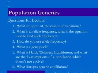
Population Genetics
Population Genetics. Outline. Allele Frequency Estimation Hardy-Weinberg equilibrium (HWE) HWE Game Population Substructure Recurrence Risk Estimation Heritability. Allele Frequency. Diploid, autosomal locus with 2 alleles: A and a Allele frequency is the fraction:.

Population Genetics
E N D
Presentation Transcript
Outline • Allele Frequency Estimation • Hardy-Weinberg equilibrium (HWE) • HWE Game • Population Substructure • Recurrence Risk Estimation • Heritability
Allele Frequency • Diploid, autosomal locus with 2 alleles: A and a • Allele frequency is the fraction: No. of particular allele No. of all alleles in population
Allele (Gamete) Frequency • Let p = Freq(A) frequency of the dominant allele • Let q = Freq(a) frequency of the recessive allele Then, p + q =1
Genotype Frequency • p2 = frequency of homozygous dominant genotype • q2 = frequency of homozygous recessive genotype • 2pq = frequency of heterozygous genotype Then, p2 +2pq + q2 =1
Estimating Allele Frequencies from Genotype Frequencies Genotypes: AA Aa aa Frequency: p2 2pq q2 • Frequency of A allele = p2 + ½ (2pq) • Frequency of a allele = q2 + ½ (2pq)
Ex. Calculation: Allele Frequencies Assume N=200 in each of two populations • Pop 1: 90 AA 40 Aa 70 aa (N=200) • Pop 2: 45 AA 130Aa 25 aa (N=200) In Pop 1: • p = 90/200 + ½ (40/200) = 0.45 + 0.10 = 0.55 • q = 70/200 + ½ (40/200) = 0.35 + 0.10 = 0.45 In Pop 2: • p = 45/200 + ½ (130/200) = 0.225 + 0.325 = 0.55 • q = 25/200 + ½ (130/200) = 0.125 + 0.325 = 0.45
Take home points • p + q =1 (sum of the allele frequencies = 1) • p2 + 2pq + q2 =1 (sum of the genotype frequencies = 1) • Two populations with markedly different genotype frequencies can have the same allele frequencies
Hardy-Weinberg The Hardy–Weinberg principle states that both allele and genotype frequencies in a population remain constant—that is, they are in equilibrium—from generation to generation unless specific disturbing influences are introduced p2 + 2pq + q2 = 1
Hardy-Weinberg Assumptions Allele frequencies do not vary IF: • Large population • Random mating • No in or out migration • No isolated groups within the population • No mutation • No selection (no allele is advantageous)
Example: Test of Hardy-Weinberg Equilibrium (HWE) • We have the following observed genotype frequencies: 100 GG, 30 AG, 20AA • Frequency of the G allele: p = 100/150 + 0.5(30/150) = 0.767 • Frequency of the A allele q = 20/150 + 0.5(30/150) = 0.233 = 1-p
Test of Hardy-Weinberg Equilibrium 2. Calculate expected genotype frequencies based on HW: p2 + 2pq + q2 = 1 GG p2 = 0.767*0.767 = 0.588 n(p2) = 150(0.588) = 88.2 AG 2pq = 2*0.767*0.233 = 0.357 n(2pq) = 150(0.357) = 53.6 AA q2 = 0.233*0.233 = 0.054 n(q2) = 150(0.054) = 8.1
Test of Hardy-Weinberg Equilibrium 3. Compare expected genotype counts (E) to observed genotype counts (O) E O(O-E)^2/E GG 88.2 100 1.58 AG 53.6 30 10.39 AA 8.1 20 17.48 ----- 29.45 Chi-square test = Σi (Oi – Ei)2/Ei = 29.4 (chi square distribution with 1 degree of freedom) p = 6.6 x 10⁻⁸ > Out of H-W
HWE can be easily expanded to account for any number of alleles at a locus • 3 allele case (p1, p2, p3) Allele frequencies: p1 + p2 + p3 = 1 Genotype frequencies: p12 + p22 + p32 + 2p1p2 + 2p1p3 + 2p2p3= 1 • 4 allele case (p1, p2, p3, p4) Allele frequencies: p1 + p2 + p3 + p4= 1 Genotype frequencies: p12 + p22 + p32 + p42 + 2p1p2 + 2p1p3 + 2p2p3 + 2p3p4= 1
Application of Hardy-Weinberg Equilibrium For genetic association studies: • Used as QC measure to assess the accuracy of the genotyping method • Expect SNPs to be in HWE among control populations (ethnic-specific) • Violations of HWE could indicate genotyping errors or bias in data
HWE Game Everyone receives ~5 pairs of cards Two allele model: Red (R allele) & Black (B allele) Random Mating: Exchange one card from each pair with another person (keep cards face down) Determine genotype frequency: RR, RB, BB Determine allele frequency: R, B
Population stratification Population stratification is a form of confounding in genetic studies where a gene under study shows marked variation in allele frequency across subgroups of a population and these subgroups differ in their baseline risk of disease
Population Stratification: Confounding Exposure of Interest Disease True Risk Factor Genotype of Interest Ethnicity True Risk Factor Disease Wacholder, JNCI, 2000
Population Stratification: Gm3;5,13,14 in admixed sample of Native Americans of the Pima and Papago tribes Study Population: 4,290 Pima and Papago Indians Genetic Variant: Gm 3;5,13, 15 haplotype (Gm system of human immunoglobulin G) Outcome: Type 2 diabetes Question: Is the Gm 3; 5,13, 15 haplotype associated with Type 2 diabetes? Knowler, AJHG, 1998
Population Stratification: Gm3;5,13,14 in admixed sample of Native Americans of the Pima and Papago tribes Unadjusted for ethnic background OR = 0.27 (95% 0.18-0.40)
Population Stratification: Gm3;5,13,14 in admixed sample of Native Americans of the Pima and Papago tribes Adjusted for ethnic background OR = 0.83 (95% 0.58-1.18)
Ancestry Informative Markers • Polymorphisms with known allele frequency differences across ancestral groups • Useful in estimating ancestry in admixed individuals • Example: Duffy locus (codes for blood group) • 100% sub-Saharan Africans vs. other groups • protects P. vivax (malaria)
Example AIM: Duffy locus (rs2814778) http://www.ncbi.nlm.nih.gov/projects/SNP
Population inbreeding Population inbreeding occurs when there is a preference of mating between close relatives or because of geographic isolation in a population. This will cause deviations in HWE by causing a deficit of heterozygotes.
How to quantify the amount of inbreeding in a population? • Inbreeding coefficient, F • The probability that a random individual in the population inherits two copies of the same allele from a common ancestor • F ranges 0 to 1: F is low in random mating populations F close to 1 in self-breeding population (plants)
Kinship & Reproduction: Icelandic couples “The first interval of kinship represents all couples related at the level of second cousins or closer, the second interval represents couples related at the level of third cousins and up to the level of second cousins, and so on, with each subsequent category representing steps to fourth, fifth, sixth, and seventh cousins and the final category representing couples with no known relationship and those with relationships up to the level of eighth cousins.” # of children # of children that reproduce # of grandchildren mean lifespan of children Helgason, Science, 2008
Process of Genetic Epidemiology Defining the Phenotype Migrant Studies Familial Aggregation Segregation Linkage Analysis Association Studies Cloning Fine Mapping Characterization
Familial Aggregation • Does the phenotype tend to run in families?
Recurrence (‘Familial’) Risk Ratios • Compares the probability a subject is affected given they have an affected family member to the population risk: R = KR/K, where KR is the risk to relatives of type R K is the population risk S = recurrence risk to siblings of probands versus the general population risk.
Recurrence Risk Ratios (RRR) R = P(Y2 = 1 |Y1 = 1) / K where Yi is individual i’s affection status P(Y2=1|Y1=1)P(Y1=1) = P(Y2=1, Y1=1) P(Y2=1|Y1=1) = P(Y2=1, Y1=1)/P(Y1=1) K = P(Y1=1) R = P(Y2=1, Y1=1)/P(Y1=1)2
Estimating RRR • With case-control data, calculate RRR as: Proportion of affected relatives of the cases (observed) / Proportion of affected relatives of controls (expected) (assumed to estimate K) Using R = P(Y2 = 1 |Y1 = 1) / K • The higher the value of R the stronger the genetic effect
Examples of s • Alzheimer Disease 3-4 • Rheumatoid Arthritis 12 • Schizophrenia 13 • Type I Diabetes 15 • Multiple Sclerosis 20-30 • Neural Tube Defects 25-50 • Autism 75-150
Limitations of recurrence risks (Figure 4.1, p. 53) • Recurrence risks depend on mode of inheritance and disease frequency. • Single gene diseases have high recurrence risks • More common complex diseases have lower values (e.g., CHD). • Here, hard to distinguish genetic versus environmental effects.
s versus Genetic Relative Risk (GRR) s =P(Y2=1|Y1=1) ? P(Y2=1|D) = GRR P(Y2=1|Y1=0) P(Y2=1|dd) Assume that D is causal for Y. Sibling’s disease (Y1) not necessarily hereditary At risk individual may not have inherited D Sib unaffected doesn’t mean other sib doesn’t carry D
Dominant (GRR, Genetic Relative Risk)
Recessive (GRR, Genetic Relative Risk)
Heritability Analysis • Evaluates the genetic contribution to a trait Y in terms of variance explained. • Y = Genetics + Environment • Var(Y) = Var(G) + Var(E) + 2Cov(G,E) = overall variation in phenotype Y
Broad Sense Heritability • Proportion of phenotypic variance that is explained by genetics: H2 = Var (G) / Var (Y) where Var(G) = genetic part of variance = VA+VD+VI VA = Additive (het between homozygotes) VD = Dominance (part beyond additive) VI = Interaction (epistatic variance, GxG)
Narrow Sense Heritability • Proportion of phenotypic variance that is explained only by additive genetic effects: h2 = VA / Var (Y) • Additive is largest part, and commonly focus only on this. • Can estimate from regression: • Additive: 0, 1, 2 for alleles • Dominance: 0, 1, 0 for departure • Interaction: product of these • Or estimate from twin studies
Twin Studies • Compare the phenotype correlation or disease concordance rates of MZ (identical) and DZ (fraternal) twins. Parents: Possible offspring
MZ Twins (Identical) If twin 1 is Both alleles are shared identical by descent (IBD) Then twin 2 must be:
DZ Twins (Fraternal) Twin 1 Twin 2: any of the four IBD can be 2, 1, or 0 2 1 1 0
DZ Twins (Fraternal) Twin 1 Average sharing is 50% 100% 50% 50% 0%
IBD Sharing # of alleles shared IBD 2 1 0 Pr(2) Pr(1) Pr(0) Prop IBD Relationship Self, MZ twins 1 0 0 1 Parent, Offspring 0 1 0 1/2 Full siblings 1/4 1/2 1/4 1/2 Gr-child, Gr-prt 0 1/4 3/4 1/4 First cousins 0 1/4 3/4 1/8 Proportion of alleles shared IBD = # alleles x Pr(# alleles) / 2
Twin Studies • ACE Model • A: Additive genetics • C: Common Environment • E: Unique Environment • Correlation in phenotype (Y1, Y2) among twins: • Corrmz(Y1, Y2) = rmz = A + C [100% genes + Env] • Corrmz(Y1, Y2) = rdz = ½A + C [50% genes + Env] • Heritability: h2 = 2(rmz- rdz )
Example of Twin Study: PCa • Twin registry (Sweden, Denmark, and Finland) 7,231 MZ and 13,769 DZ Twins (male) Heritability = 2(rmz- rdz ) = 2(0.21-0.06) = 0.30 Lichtenstein et al NEJM 2000 13;343:78-85. (actual paper estimate uses Structural Equation Modeling, so differs) Limitations of heritability calculations?
Segregation Analysis • Study families. • Estimate ‘mode of inheritance’ & what type of genetic variant might be causal. • Determine whether the disease appears to follow particular patterns across generations. • Estimate whether variants are rare or common, etc.