Download
1 / 55
570 likes | 791 Vues
Ultrasound. Ultrasound. History. 1880 Curies discover piezoelectric effect 1914-1918 Langevin begins development of SONAR 1928 Sokolov applies to crack detection 1930 Medical therapy eg cancer 1940s Medical Diagnostic- SONAR. Wave Characteristics I.

E N D
History • 1880 Curies discover piezoelectric effect • 1914-1918 Langevin begins development of SONAR • 1928 Sokolov applies to crack detection • 1930 Medical therapy eg cancer • 1940s Medical Diagnostic- SONAR
Wave Characteristics I Longitudinal Compression & Rarefaction wave. eg A Sound Wave • Propagates in solid, liquid or gas • Frequency fixed by transmitter Infrasound frequency < 20 Hz Sound 20 Hz < frequency < 20,000 Hz Ultrasound frequency > 20,000 Hz Medical ultrasound 1 MHz < frequency < 20MHz
Wave Characteristics II Velocity is fixed by medium velocity = in a solid velocity = in a fluid velocity = in a gas The speed of sound is temperature sensitive!
Velocities in Selected Media Non-Biological Velocity (m/sec) Biological Velocity (m/sec) Air 331 Acetone 1174 Fat 1475 Ethanol 1207 Soft tissue 1540 Water 25C 1498 Brain 1560 Mercury 1450 Kidney 1560 Water 50C 1540 Spleen 1570 Polyethylene 1950 Liver 1570 Nylon(6-6) 2620 Blood 1570 Acrylic plastic 2680 Muscle 1580 Brass 4700 Eye lens 1620 Glass 5640 Skull bone 3360 Aluminium 6420
Wavelength Set by frequency at source n and velocity in the medium c c = l n In soft tissue c = 1540 and n = 1MHz wavelength = 1.54mm • suitable for imaging
Intensity is measured in W/m2 power per square metre For a pressure wave I = since m = p V I = 2 p2p n2 R2 where R = amplitude of the motion I =
Decibels are logarithmic intensities I (dB) = 10 log where Io = 10-12 W/m2 I (dB) = 10 log where Po = 10-12 W/m2 = 20 log
Acoustic field parameters What are the longitudinal displacement velocity accelerations of tissue? for normal ultrasound pulse of peak intensity 2 x 10⁵ W/m2 Peak displacement 8 x 10⁻⁸ m Peak velocity 0.5m/s Longitudinal acceleration 3 x 10⁶ m/s2 Peak pressures 8 atm.
Attenuation For a small slab width dx and attenuation coefficient m m-1 dI = m I dx I = Io exp ( - m x)
Attenuation Attenuation in medical ultrasound: 1: Increases nearly linearly with frequency 2: Amplitude attenuation a ( dB/cm/MHz)approx = 1 3: Contains both absorption and scattering terms. scattered = 10%to 30% of total
Ultrasonic properties of materials Absorption Conversion of wave energy to heat through: 1: Classical Viscous losses: proportional to n2 frequency Little effect in tissue 2: Molecular relaxation: proportional to n frequency pressure and temperature variations cause reversible change in molecular structure. Dominant in tissue ( except lung and bone) 3: Relative motion losses: Viscous or thermally damped Generally High Protein content or low water content means high absorption
Ultrasonic properties of materials Scattering Tissues with sizes from Cells 10 microns [ 0.03 l at 5 MHz] Rayleigh scattering proportional to n4 weak and predominantly backward Intermediate 300 microns [ 1l at 5 MHz] Stochastic scattering variable frequency dependence somewhat forward but variable Organ boundaries 10cm [ 300 l at 5 MHz ] Geometric scattering eg reflection
q q r i incident reflected wave wave refracted wave t q Reflection & Refraction Reflection qi = qr Refraction sin qi /sin qt = n
Impedance Acoustic Impedance = p c = density x velocity
q q r i incident reflected wave wave q t Reflection and refraction Normal Incidence Intensity of the reflected and transmitted sound: R+T =1
Transmission in Tissues a ( dB/cm/MHz)approx = 1
Impedance matching If Z1 = Z2 Matched impedance R is small T is large. The forward transmitted intensity is high. If Z1 >> Z2 Impedance mismatch R > T and the reflected intensity is high. eg Air-tissue interface
Z1 Z2 X1 X2 Engineering Principles Key Functions: 1: Send pulse train 2:Pulse train is reflected from interfaces 3: Pulse train is received 4: Cycle is repeated Distance to structure = time of flight
Dt pulse duration Pulse Separation Returned Pulses from one cycle must not overlap into the next cycle. Maximum distance imaged = 1/2 CaveDt where Cave is the average velocity in tissue= 1540 m/s Dt is the time between cycles or pulse separation For a range of 10cm Dt = 2 x 10x10-2/1540 = 1.3 x 10 -4 sec For a 1MHz ultrasound the pulse wavelength is 1.54 mm Pulse duration is usually 1 cycle T = 10-6 sec Pulse Repetition Rate ( KHz) =
Transducers Three components 1: piezoelectric element Generates pressure pulse Detects pressure pulse 2: backing material Absorbs reverse wave Damps vibration between pulses 3: electrically screened casing
+ - + - + - + - + - + - + - + - + - + - + - + - + - + - + - + - + - + - no voltage applied voltage Piezo Element Ceramic PZT ( lead zirconate/ BaTiO3) Acoustic impedance = 30 Plastic PVD polyvinylidine difluoride new copolymers allow flexible film PVD Acoustic impedance = 2.7 • Applied voltage aligns dipoles in PZT and crystal expands • Crystal can vibrate in thickness mode or radial mode
thickness 1/2 wavelength Transducer Resonant Frequency Resonant frequency: Fundamental mode is at a wavelength l = 2 * thickness Wave from the back surface reinforces front surface wave PZT-4 1mm thick c = 4000 m/s in crystal l = 2x 10⁻³ m n = 2 MHz
Curie Temperature Temperature above which PZT loses its properties. Quartz 573 C Barium Titanate 100 C PZT-4 328 C You cannot sterilise ultrasound head using an autoclave!
low Q high Q relative amplitude f1 fo f2 frequency The Quality Factor Q The sharpness of the frequency response curve Q = fo/(f2-f1) where f1 and f2 are the half power points
Transducer Construction Ring Down time: The interval between initiation of the pulse and its cessation High Q transducers have a long ring down time. The Q factor of transducers is controlled by the backing block which quenches the vibration and shortens the pulse. The backing block: Attenuates reverse wavefront Stops reflected wave interfering with front surface wave since this would lengthen pulse. Usually tungsten and rubber powder in epoxy resin. Tungsten and rubber ratio satisfies impedance matching Epoxy attenuates sound. Matching Layer: PZT acoustic impedance >> tissue impedance Matching layer thickness = l/4 Z2 = (ZPZT* Ztissue)2 example, Aluminium powder in araldite PZDs do not need a matching layer
Wavefronts and Near Fields Fresnel zone q 2r Fraunhofer zone Fresnel or Near Field Zone D Fresnel = radius2/l Close to the source the wavelets are highly circular Interference effects dominate The beam width is no greater than the diameter of the transducer. Fraunhofer or Far Field Zone Beyond the Fresnel distance the beam gradually diverges sin q = 1.22l/ transducer diameter Medical ultrasound requires a large Fresnel zone. For f = 2MHz and r = 10mm DFresnel = 13cm
Focussed Beams 1: Concave crystals 2: Mirrors 3: Lenses Velocity is greater in lens than medium. Concave lens focuses focal zone or depth of focus = 10 l (f/diameter ) 2 4: Zone plates • Diffraction effects
Scanning systems Mechanical Encoders The angle of the beam to the vertical is sensed electro-mechanically
delay lines short ……..long Transducer Arrays 1: Scanning by sweeping a linear array 2: Phased arrays Beam Steering Delay lines in circuits driving each element scan the beam. Dynamic focussing Delays in circuits to each element phased to produce converging wavefront.
3-D Scanning With the advent of fast computers three-dimensional images are now possible byperforming a sequence of overlapping two-dimensional scans offset at right angles tothe scan direction.
"A" and "B" Type Displays A-Mode intensity of returned signal v time Real time display with no memory Brightness-modulated (B) mode • Each echo is represented by a bright spot on the oscilloscope. • The amplitudeof the echo is proportional to the brightness of thespot. • The position of the spotrepresents the position of the interface at which the ultrasound was reflected, as in the A scan.
Imaging B Mode B- Mode ImagingImages slice of tissue Images can be built up by scanning the beam and using memory or persistent screen
Variations with time (M & TM) M-ModeDepth varies with time Development of B-mode with a fixed beam Used to study moving structures eg echocardiography No memory TM-Mode Depth varies with time Persistent display or memory displays as graph. Possible use of strip chart recorder.
Two-dimensional scan • Two-dimensional images can be produced by tilting the transducer probe to slowly scan a 2-D region shaped rather like a fan. • The information is stored point by point on an storage oscilloscope or in a computer memory and displayed as a two-dimensional picture. • A computer can translate the collected information in to a clearer, more colourful and detailedimage.
Digital Systems Components: Clock pulses triggers excitation of transducer synchronises send/receive synchronises display Transmitter Applies pulse to transducer ( pulser) 100V < voltage < 200V Pulse rise times < 25 ns @ 10MHz Linear RF amplifier Low noise & high gain Short recovery time Large dynamic range Good linearity
Preprocessing Before signal is sent to display memory • Attenuator Coarse system gain control • Time gain control Attenuation controlled by arrival time Echos from distant sources are highly attenuated. Set by potentiometers [ sliders] or control knobs Near gain and delay set gain for near echoes TGC sets slope for amplification- depth Enhancement windows specific depth range for increased amplification Far gain enhances all distant echoes
Filtering and Demodulation Compression Filter Allows high dynamic range to be imaged ie 40dB to 50dB Non linear stretch eg log amplifier Demodulation Envelope of RF signal extracted Digitisation Conversion of voltage to stored display value. 0- 30dB mapped onto 0- 256 grey levels
Quality Assurance We measure: Deadzone –distance at which TGC is set to zero Axial resolution- depth resolution Lateral resolution- horizontal resolution Horizontal calibration Vertical Calibration Heggie Liddel and Maher
Deadzone Phantom Display TGC Dead zone 10% ethanol in water V = 1540 m/s Nylon filaments
Axial Resolution Phantom Display unresolved
unresolved Lateral resolution Phantom Display Horizontal and Vertical Calibration Markers at known vertical and lateral spacings. Calibration errors will arise if calibrated sound speed differs from phantom
Artifacts Image reconstruction assumes: Speed of sound in tissue is constant 1540 m/s All echos detected are due to a single reflection from the beam’s central axis The beam travels in a straight line Attenuation is constant with depth These assumptions can be violated and lead to Multiple reflections Acoustic shadowing Misregistration Enhancement Mirror imaging
Reverberation & Multiple Refelction Heggie Liddel and Maher
Multipath Reflection Heggie Liddel and Maher