Blocking Phenomenon in Psychology
E N D
Presentation Transcript
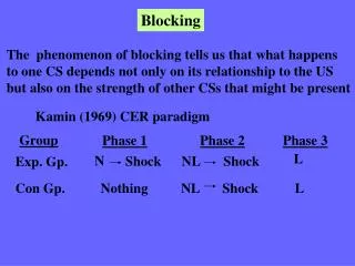
Blocking The phenomenon of blocking tells us that what happens to one CS depends not only on its relationship to the US but also on the strength of other CSs that might be present Kamin (1969) CER paradigm Group Phase 1 Phase 2 Phase 3 L N Shock NL Shock Exp. Gp. Con Gp. Nothing NL Shock L
Results (CR to L) .5 .4 Supp. ratio .3 .2 .1 0 Con Exp Learning to the added cue (L) is blocked by prior conditioning with the N See little CR to L in Experimental group because the N is already a good predictor of the US
The concept of surprise is important in explaining the Blocking effect Conditioning only occurs if the animal is surprised by the US T US On the first trial, the animal doesn’t expect the US The US is surprising and learning takes place Over trials the animal learns that the T predicts the US The US is no longer surprising and the rate of learning slows down
6 5 4 3 2 1 5 6 7 8 2 1 4 9 10 11 12 3 Typical Learning Curve asymptote
On compound trials, give LT US Get little or no conditioning to the new L because the US is not surprising; it is predicted by the T The L is redundant; it provides no new information What would happen if you changed the US on compound trials? The US would now be surprising, so should see conditioning to the added cue Unblocking Unblocking is the elimination of the blocking effect – see learning to the new cue
Holland demonstrated unblocking by changing the US (increased and decreased the US in separate groups) This experiment demonstrates the importance of surprise 4 groups of rats Phase 1 Phase 2 (1-1) = no surprise L 1 pellet LN 1 pellet L 1 pellet LN 3 pellets (1-3) = surprise L 3 pellets LN 1 pellet (3-1) = surprise L 3 pellets LN 3 pellets (3-3) = no surprise 2 groups received the same # of pellets in phases 1 and 2 (blocking) 2 groups received a change in the number of pellets (unblocking)
Results Unblocking (see learning To N) (1-3) (3-1) % CR to N Blocking (no learning To N) (3-3) (1-1) Test sessions
The Rescorla-Wagner Model • Based on the concept of surprise • better than simple contingency theory Contingency theory Associations develop when a subject assesses the correlation or predictive relationship between the CS and US Excitatory conditioning occurs when: p(US/CS) > p(US/no CS) Problem with contingency theory is that it doesn’t take into consideration what is happening to other CSs; therefore, it can’t explain blocking
The Rescorla-Wagner Model • mathematical model • US processing model • conditioning depends on the degree to which the • US is processed • according to the model, each US has a certain amount • of associative strength that will support conditioning • takes into account all the CSs present on a given trial • the concept of surprise is important to the RW model • surprise is defined as the discrepancy between the US • that is expected and the one that actually occurs
The Rescorla-Wagner Model Should be able to grasp the general idea of the RW model if you understand the following 6 basic rules: • If the strength of the actual US is greater than the • strength of the subject’s expectation, all CSs that are • paired with the US will receive excitatory conditioning • If the strength of the actual US is less than the strength • of the subject’s expectation, all CSs that are paired with • the US will receive some inhibitory conditioning 3. If the strength of the actual US is equal to the strength of the subject’s expectation, there will be no conditioning
The Rescorla-Wagner Model • The larger the discrepancy between the strength of • the expectation and the strength of the US, the greater • will be the conditioning (either excitatory or inhibitory) • that occurs • More salient CSs will condition faster than less salient • CSs • If 2 or more CSs are presented together, the subject’s • expectation will be equal to their total strength (with • excitatory and inhibitory stimuli tending to cancel each • other out)
Acquisition L 1 pellet of food Trial 1: Rat has no expectation of the US So, the strength of the US is much greater than the rat’s expectation (which is ‘0’) Therefore, this trial produces some excitatory conditioning (refer to Rule #1) But conditioning is rarely complete after 1 trial Trial 2: The second time the L is presented, it will elicit some expectation of the US, but still not as strong as the actual US So rule #1 applies again and more excitatory conditioning develops – and so on for trials 3, 4, 5……
Acquisition L 1 pellet of food At each conditioning trial, the rat’s expectation of the food pellet should get stronger The difference between the strength of the expectation and the strength of the US gets smaller The fastest growth in conditioning occurs on the first few trials and there is less and less conditioning as the trials proceed (rule #4) Eventually, the L elicits an expectation of 1 pellet and 1 pellet is given – the asymptote of learning is reached and no further conditioning occurs
6 5 4 3 2 1 5 6 7 8 2 1 4 9 10 11 12 3 Learning Curve The RW model predicts the typical learning curve (acquisition)
Blocking Now, suppose asymptote is reached and we give: LT 1 pellet of food According to rule #6, when 2 CSs are presented the subject’s expectation is based on the total expectation from the 2 CSs T is a new stimulus = ‘0’ expectation L produces expectation of 1 pellet The actual US = 1 pellet; expectation matches the US that is given and no additional conditioning occurs (rule #3) The L retains its excitatory strength and the T retains its ‘0’ strength
The Rescorla-Wagner Model ΔV = k(λ – V) Δ = change so ΔV = change in the strength of the CS k = constant Related to the salience of the CS and US Refers to the associability of the CS λ = maximum amount of conditioning that the US can support – its our actual US value λ – V = the discrepancy between what the animal expects (V) and the actual US that is given (λ)
The Rescorla-Wagner Model Will sometimes see the formula written as: ΔVA = k(λ – VT) ΔVA = change in the strength of CSA VT = strength of all CSs on a given trial (VT = VA + VB …..)
ΔVA = k(λ – VT) Pair CSA Food for 5 trials VT = VA; since only 1 CS k = 0.5; constant λ = 100; US Trial 1: ΔVA = k(λ – VT) ΔVA = 0.5 (100 – 0) = 50 So, change in strength of CS is 50 units Trial 2: ΔVA = 0.5 (100 – 50) = 0.5 (50) = 25 CS gains additional 25 units
ΔVA = k(λ – VT) Trial 3: ΔVA = 0.5 (100 – 75) = 0.5 (25) = 12.5 Trial 4: ΔVA = 0.5 (100 – 87.5) = 0.5 (12.5) = 6.3 Trial 5: ΔVA = 0.5 (100 – 93.8) = 0.5 (6.2) = 3.1 ΔVA across 5 trials: 50 + 25 + 12.5 + 6.3 + 3.1 = 96.9 With more trials, V = λ = 100
Most conditioning occurs on trial 1 (50 units) On subsequent trials the CS acquires additional strength which is a fixed proportion of the strength that is still available As conditioning progresses, the discrepancy between the expected and actual US declines; (λ – VT) gets smaller So, the RW model predicts the typical learning curve
100 80 60 40 20 1 2 3 4 5 6 Learning Curve VCS or CR Trials
Rescorla-Wagner Model and Blocking At the end of trial 5, in the previous example, the total strength of all CSs is 96.9 (VT = VA = 96.9) This means 3.1 units from the original 100 are available on trial 6 Trial 6: ΔV = k(λ – VT) Food CSA/CSB ΔVB = .5 (100-96.9) Assume k = .5 VT = VA + VB = .5 (3.1) = 1.5 Recall, CSA on first trial gained 50 units of strength But, CSB gained only 1.5 units of strength Conditioning to CSB is blocked
The RW model can explain acquisition and blocking The RW model can also explain extinction and conditioned inhibition ΔVA = k(λ – VT) Suppose after asymptote is reached with L-Food pairings we give: Assume k = .5 VA = 100 (asymptote) LT No food Here, rule #2 applies: The strength of the expectation will exceed the strength of the actual US λ = 0 (no US is given); VT = 100, because L is given
According to rule #2, both CSs will acquire some inhibitory strength How does this inhibitory conditioning affect the L and T? Because the L starts with strong excitatory strength, the trials without food and the inhibitory conditioning they produce will begin to counteract this excitatory strength This is an example of extinction – presenting the CS without the US ΔVA = .5(0-100) = -50 ΔVA = k(λ – VT) L starts with 100, now reduced to 50 – but still excitatory Repeated trials without the US would reduce L to ‘0’
Remember, L food (until asymptote) Then, LT no food The T begins this phase with ‘0’ strength because it hasn’t been presented before Therefore, trials without food will cause the strength of the T to decrease below 0 – it will become a CI ΔVA = .5(0-100) = -50 ΔVA = k(λ – VT) T starts with 0, now at –50; so its inhibitory
The RW model can also explain the US-pre-exposure effect Phase 1: US alone Phase 2: CS US pairings On US alone trials, the background cues become conditioned Then when CS-US trials are given, it becomes a blocking experiment US Context + CS
Unusual prediction of the RW Model Loss of associative value despite pairings with the US Phase 1: Phase 2: A US A + B US B US A and B are trained to asymptote in phase 1 Then in phase 2, both CSs are presented together with the same US The expectation in phase 2, would be 2X the US However, only 1 US is given, so the expectation exceeds the actual US So, should see a decrease in CR to both A and B
Evaluation of the RW Model The RW model cannot account for latent inhibition (LI) Phase 1: CS alone Phase 2: CS US pairings According to the model the CS should not gain or lose strength when no US is present The RW Model is a US-processing model So, change in strength of CS on first trial is ‘0’ ΔVA = k(λ – VT) The next trial would be the same ΔVA = .5(0 – 0) = 0 No increase or decrease in strength of the CS
Evaluation of the RW Model Another problem for the model is unblocking There are 2 types of unblocking: Unblocking with an upshift (i.e., the US is increased) Unblocking with an downshift (i.e., the US is decreased) The RW model can explain unblocking with an upshift If the US is increased, λ is increased, there is room to see conditioning to the added CS The model cannot explain unblocking with a downshift If the US is decreased, λ is decreased. Should never see excitatory conditioning to the added CS
Evaluation of the RW Model Extinction According to the model, extinction should reduce the strength of the CS to ‘0’ i.e., extinction is the reverse of acquisition However, we know that extinction is the not the reverse of acquisition Spontaneous Recovery: if we give the animals a rest period, responding the CS recovers Temporal factors in conditioning Temporal factors like the CS-US interval are important but the RW Model cannot account for these factors

