Download
1 / 26
260 likes | 489 Vues
The AS-AD model. Aggregate Demand Aggregate Supply Policy analysis. The AS-AD model. Week 6: we examined how monetary and fiscal policy affect aggregate demand, by using different combinations of the policy mix Remember that 2 assumptions were made:

E N D
The AS-AD model Aggregate Demand Aggregate Supply Policy analysis
The AS-AD model • Week 6: we examined how monetary and fiscal policy affect aggregate demand, by using different combinations of the policy mix • Remember that 2 assumptions were made: • There exists excess production capacity in the economy (unemployment, under-utilised capital) • The price of goods, services and factors of production are fixed and do not adjust • These assumptions can be restrictive and create some problems
LM LM’ LM’’ Interest rate i i2 i1 IS’ IS’’ IS Income, Output Y Y1 Y2 The AS-AD model 1. Using the correct policy mix allows you to increase output and keep interest rates relatively constant To infinity and beyond... 2. But what’s to stop you going on for ever ??
The AS-AD model • Intuitively, we know there is a limit to IS-LM: • As we’ve seen, in IS-LM, you can boost GDP forever using the Policy-mix • In real life, one knows that over-using these policies leads mainly to inflation. • Why the difference? Where does this inflation come from ? • Bottom line: if demand increases beyond the productive capacity of the economy, producers have no choice but to increase prices • The purpose of the AS-AD model is to correct the predictions of IS-LM in order to account for the fact that there is not always excess productive capacity.
The AS-AD model • Modelling strategy Money market equilibrium Keynesian Equilibrium IS Curve LM Curve Labour market Equilibrium IS-LM model Aggregate supply curve Aggregate demand curve Model of macroeconomic fluctuations
The AS-AD model The Aggregate Demand curve The Aggregate Supply curve The AS-AD equilibrium
The AD curve • The AD curve shows the amount of goods and services demanded for a given price level. • The AD curve has a negative slope : a lower level of prices tends to increase the aggregate demand for goods and services • Prices affect the LM curve through real money balances: a higher price level leads to higher interest rates in IS-LM, reducing equilibrium output. • Beware: The negative slope of the AD curve isNOTlinked to the negative slope of micro demand curves!!
i i LM’ LM L2(Y) Y L1(Y) L1(Y) L2(Y) Y The AD curve This shifts LM left L2(i) An increase in prices reduces real money balances (M/P) L1(Y) (M/P) = L1(Y) + L2(i) 45° 45°
P Y The AD curve 3. However, a reduction in M at constant price leads to a shift in AD 2. The AD curve plots this overall effect P P2 P1 P1 AD AD AD’ Y LM2 LM’ i i LM1 LM1 i2 i2 i1 i1 1. An increase in the price level from P1 to P2 reduces real money balances, which shifts LM IS IS Y Y Y2 Y2 Y1 Y1
P Y The AD curve • Rules of thumb: • A shift in IS • Always leads to a similar shift in AD • A shift in LM • Leads to a similar shift in AD only if the shift is not due to changes in the price level • Changes in the price level bring movement on AD 2. Because prices are unchanged, this leads to a shift of the AD curve P1 AD’ AD LM2 1. An increase in government spending shifts IS to the right, increasing output and interest rates i i i2 i1 IS’ IS Y Y1 Y2
The AS-AD model The Aggregate Demand curve The Aggregate Supply curve The AS-AD equilibrium
The AS curve • The AS curve shows the amount of goods and services supplied for a given price level. • Compared to the AD curve, one has to distinguish between the short run AS (SRAS) and the long run AS (LRAS): • LRAS : In the long run, the productive capacity of the economy does not depend on prices • SRAS : A change in prices changes the real cost of labour, affecting the productive capacity of the economy. • Beware: The positive slope of the SRAS curve is NOT linked to the slope of micro supply curves !!
The AS curve • The short run AS is derived from the WS-PS/Phillips curve framework we examined in the previous weeks. • The Phillips curve already identifies a negative trade-off between unemployment and inflation. • But what we need is a trade-off between prices/inflation and output • So how do we bridge this gap ? • We use Okun’s law, the empirical relation between output and unemployment
inflation rate π β Πe Unemployment rate u un The AS curve Reminder of the Phillips curve 1
The AS curve • Okun’s Law:
The AS curve • The Phillips curve is the negative empirical relation between inflation and unemployment (It can be obtained with the WS – PS model) : • Okun’s law is a similar negative empirical relation : • Disregarding the random shocks, one can combine these two to obtain a short run aggregate supply (SRAS) equation: Negative Relations Positive Relation
inflation rate π inflation rate π β γ Πe Unemployment rate u Y n un Output Y The AS curve 1 1
The AS curve π LRAS In the long run, π* = π e, and the economy is at its potential output Yn, which corresponds to the natural rate of unemployment un. SRAS If a shock increases prices, then the real cost of labour W/P will drop, pushing output Y above potential output and unemployment u below the natural rate. π’ π * Workers will adjust their expectations π e and negotiate higher nominal wages. This increases the real labour costs and shifts the SRAS to the left, until the long run equilibrium is reached again Yn Y Y
LRAS Yn The AS curve π The long run aggregate supply is vertical at Yn. This means that the Y=Yn condition is equivalent to u=un and π = π e Fall in LRAS Increase in LRAS This does NOT mean that the potential level of output Yn is fixed in time It means that Yn is a function of other variables than price Y
The AS-AD model The Aggregate Demand curve The Aggregate Supply curve The AS-AD equilibrium
The AS-AD equilibrium π LRAS SRAS In the long run macroeconomic equilibrium, price expectations are fulfilled (π* = π e), and demand in the economy is equal to the long run productive capacity (Y =Yn). π * AD Yn Y
The AS-AD equilibrium • Shocks to demand and supply lead to fluctuations at the macroeconomic level. • By “shocks” economists mean exogenous variations to supply and demand • A demand shock modifies aggregate demand: increase in G or T, change in M, etc. • A supply shock modifies aggregate supply: increase in oil prices, change in technology, etc. • Stabilisation policies are policies that attempt to keep output, inflation and employment around their long run equilibrium levels • The aim is to minimise the fluctuations around equilibrium
A negative demand shock shifts the AD curve to the left, which reduces output and prices SRAS2 Supply-side policy: Stimulate the SRAS by reducing the effective cost of factors (wages) and get to C B π 1 C π 2 AD2 Y1 The AS-AD equilibrium π LRAS SRAS How can we return to the long run equilibrium ? A π * Demand-side policy : Stimulate AD with an IS-LM policy-mix to return to point A. Preferred solution as it stimulates a depressed demand. Consistent with the IS-LM framework AD Yn Y
SRAS2 π 2 π 1 AD2 Y1 The AS-AD equilibrium A negative supply shock (increase in production costs) causes an increase in prices and a fall in output in the short run: This is called stagflation π LRAS SRAS Demand-side policy : A demand-side policy can avoid the recession, but at the cost of high inflation: this is what happened in the late 70’s π * Supply-side policy: It is preferable to carry out a supply-side policy aiming to increase the SRAS, through a reduction of inflation expectations and a policy of wage moderation. AD Yn Y
The AS-AD equilibrium • The AS-AD model allows a better understanding of how to coordinate stabilisation policies • The best response to a demand shock is a demand policy (such as a fiscal stimulus policy) • The best response to a supply shock is a supply side policy (such as wage moderation and reduction of inflation expectations)