Download

1 / 30
300 likes | 394 Vues
Formal Biology of the Cell Modeling, Computing and Reasoning with Constraints François Fages, Constraint Programming Group, INRIA Rocquencourt mailto:Francois.Fages@inria.fr http://contraintes.inria.fr/. Overview of the Lectures. Introduction. Formal molecules and reactions in BIOCHAM.

E N D
Formal Biology of the CellModeling, Computing and Reasoning with ConstraintsFrançois Fages, Constraint Programming Group, INRIA Rocquencourtmailto:Francois.Fages@inria.frhttp://contraintes.inria.fr/
Overview of the Lectures • Introduction. Formal molecules and reactions in BIOCHAM. • Formal biological properties in temporal logic. Symbolic model-checking. • Continuous dynamics. Kinetics models. • Computational models of the cell cycle control [L. Calzone]. • Mixed models of the cell cycle and the circadian cycle [L. Calzone]. • Machine learning reaction rules from temporal properties. • Constraint-based model checking. Learning kinetic parameter values. • Constraint Logic Programming approach to protein structure prediction.
Biochemical Kinetics • Study the concentration of chemical substances in a biological system as a function of time. • BIOCHAM concentration semantics: • Molecules: A1 ,…, Am • |A|=Number of molecules A • [A]=Concentration of A in the solution: [A] = |A| / Volume ML-1 • Solutions with stoichiometric coefficients: c1 *A1 +…+ cn * An
Law of Mass Action • The number of A+B interactions is proportional to the number of A and B molecules, the proportionality factor k is the rate constant of the reaction • A + B k C • the rate of the reaction is k*[A]*[B]. • dC/dt = k A B • dA/dt = -k A B • dB/dt = -k A B • Assumption: each molecule moves independently of other molecules in a random walk (diffusion, dilute solutions, low concentration).
Interpretation of Rate Constants k’s • Complexation: probabilities of reaction • upon collision (specificity, affinity) • Position of matching surfaces • Decomplexation: energy of bonds • (giving dissociation rates) • Different diffusion speeds (small molecules>substrates>enzymes…) • Average travel in a random walk: 1 μm in 1s, 2μm in 4s, 10μm in 100s • For an enzyme: • 500000 random collisions per second for a substrate concentration of 10-5 • 50000 random collisions per second for a substrate concentration of 10-6
Signal Reception on the Membrane present(L,0.5). present(RTK,0.01). absent(L-RTK). absent(S). parameter(k1,1). parameter(k2,0.1). parameter(k3,1). parameter(k4,0.3). (k1*[L]*[RTK], k2*[L-RTK]) for L+RTK <=> L-RTK. (k3*[L-RTK], k4*[S]) for 2*(L-RTK) <=> S.
Michaelis-Menten Enzymatic Reaction • An enzyme E binds to a substrate S to catalyze the formation of product P: • E+S k1 C k2 E+P • E+S km1 C • compiles into a system of non-linear Ordinary Differential Equations • dE/dt = -k1ES+(k2+km1)C • dS/dt = -k1ES+km1C • dC/dt = k1ES-(k2+km1)C • dP/dt = k2C
Michaelis-Menten Enzymatic Reaction • An enzyme E binds to a substrate S to catalyze the formation of product P: • E+S k1 C k2 E+P • E+S km1 C • compiles into a system of non-linear Ordinary Differential Equations • dE/dt = -k1ES+(k2+km1)C • dS/dt = -k1ES+km1C • dC/dt = k1ES-(k2+km1)C • dP/dt = k2C • After simplification, supposing C0=P0=0, we get E=E0-C,
Michaelis-Menten Enzymatic Reaction • An enzyme E binds to a substrate S to catalyze the formation of product P: • E+S k1 C k2 E+P • E+S km1 C • compiles into a system of non-linear Ordinary Differential Equations • dE/dt = -k1ES+(k2+km1)C • dS/dt = -k1ES+km1C • dC/dt = k1ES-(k2+km1)C • dP/dt = k2C • After simplification, supposing C0=P0=0, we get E=E0-C, S+C+P=S0,
Michaelis-Menten Enzymatic Reaction • An enzyme E binds to a substrate S to catalyze the formation of product P: • E+S k1 C k2 E+P • E+S km1 C • compiles into a system of non-linear Ordinary Differential Equations • dE/dt = -k1ES+(k2+km1)C • dS/dt = -k1ES+km1C • dC/dt = k1ES-(k2+km1)C • dP/dt = k2C • After simplification, supposing C0=P0=0, we get E=E0-C, S+C+P=S0, • dS/dt = -k1(E0-C)S+km1C • dC/dt = k1(E0-C)S-(k2+km1)C
Multi-Scale Phenomena Hydrolysis of benzoyl-L-arginine ethyl ester by trypsin present(En,1e-8). present(S,1e-5). absent(C). absent(P). (k1*[En]*[S],km1*[C]) for En+S <=> C. k2*[C] for C => En+P. parameter(k1,4e6). parameter(km1,25). parameter(k2,15). Complex formation 5e-9 in 0.1s Product formation 1e-5 in 1000s
Numerical Integration Methods • System dX/dt = f(X). Initial conditions X0 • Idea: discretize time t0, t1=t0+Δt, t2=t1+Δt, … and compute a trace • (t0,X0,dX0/dt), (t1,X1,dX1/dt), …, (tn,Xn,dXn/dt)… • (providing a linear Kripke structure for model-checking…) • Euler’s method: ti+1=ti+ Δt • Xi+1=Xi+f(Xi)*Δt • error estimation E(Xi+1)=|f(Xi)-f(Xi+1)|*Δt • Runge-Kutta’s method: averaged intermediate computations at Δt/2 • Adaptive step method: Δti+1= Δti/2 while E>Emax, otherwise Δti+1= 2*Δti • Rosenbrock’s stiff method: solve Xi+1=Xi+f(Xi+1)*Δt by formal differentiation
Quasi-Steady State Approximation • After short initial period, the complex tends quickly to a limit. • Assume dC/dt=0
Quasi-Steady State Approximation • After short initial period, the complex tends quickly to a limit. • Assume dC/dt=0 • From dC/dt = k1S(E0-C)-(k2+km1)C • we get C = k1E0S/(k2+km1+k1S)
Quasi-Steady State Approximation • After short initial period, the complex tends quickly to a limit. • Assume dC/dt=0 • From dC/dt = k1S(E0-C)-(k2+km1)C • we get C = k1E0S/(k2+km1+k1S) • = E0S/(((k2+km1)/k1)+S) • = E0S/(Km+S) • where Km=(k2+km1)/k1
Quasi-Steady State Approximation • After short initial period, the complex tends quickly to a limit. • Assume dC/dt=0 • From dC/dt = k1S(E0-C)-(k2+km1)C • we get C = k1E0S/(k2+km1+k1S) • = E0S/(((k2+km1)/k1)+S) • = E0S/(Km+S) • where Km=(k2+km1)/k1 • dS/dt = -dP/dt • = -k2C • = -VmS / (Km+S) • where Vm= k2E0.
Quasi-Steady State Approximation • Assuming dC/dt=0, hence dE/dt=0 and C= E0 S / (Km+S). • Michaelis-Menten rate: dP/dt = -dS/dt = VmS / (Km+S) (reaction velocity) • Vm=k2*E0 • Km=(km1+k2)/k1
Quasi-Steady State Approximation • Assuming dC/dt=0, hence dE/dt=0 and C= E0 S / (Km+S). • Michaelis-Menten rate: dP/dt = -dS/dt = VmS / (Km+S) (reaction velocity) • Vm=k2*E0 (maximum velocity at saturating substrate concentration) • Km=(km1+k2)/k1
Quasi-Steady State Approximation • Assuming dC/dt=0, hence dE/dt=0 and C= E0 S / (Km+S). • Michaelis-Menten rate: dP/dt = -dS/dt = VmS / (Km+S) (reaction velocity) • Vm=k2*E0 (maximum initial velocity) • Km=(km1+k2)/k1 (substrate concentration with half maximum velocity) • Experimental measurement: • The initial velocity is • linear in E0 • hyperbolic in S0
Quasi-Steady State Approximation • Assuming dC/dt=0, hence dE/dt=0 and C= E0 S / (Km+S). • Michaelis-Menten rate: dP/dt = -dS/dt = VmS / (Km+S) (reaction velocity) • Vm=k2*E0 • Km=(km1+k2)/k1 • BIOCHAM syntax • macro(Vm, k2*[En]). • macro(Km, (km1+k2)/k1). • macro(Kf, Vm*[S]/(Km+[S])). • Kf for S =[En]=> P.
BIOCHAM Concentration Semantics • To a set of BIOCHAM rules with kinetic expressions ei • {ei for Si=>S’i}i=1,…,n • one associates the system of ODEs over variables {A1,, Ak} • dAk/dt=Σni=1ri(Ak)*ei - Σnj=1lj(Ak)*ej • where ri(A) (resp. li(A)) is the stoichiometric coefficient of A in Si (resp. S’i). • Note on compositionality: The union of two sets of reaction rules is a set of reaction rules… So in principle BIOCHAM models can be composed to form complex models by simple set union.
Compositionality of Reaction Rules • Towards open modular models: • Sufficiently decomposed reaction rules, • E+S<=>C =>E+P, not S<=[E]=>P if competition on C • Sufficiently general kinetics expression, • parameters as possibly functions of temperature, pH, pressure, light,… • different pH=-log[H+] in intracellular and extracellular solvents (water) • Ex. pH(cytosol)=7.2, pH(lysosomes)=4.5, pH(cytoplasm) in [6.6,7.2] • Interface variables, • controlled either by other modules (endogeneous variables) • or by fixed laws (exogeneous variables).
Competitive Inhibition • present(En,1e-8). present(S,1e-5). • (k1*[En]*[S],km1*[C]) for En+S <=> C. k2*[C] for C => En+P. • parameter(k1,4e6). parameter(km1,25). parameter(k2,15). • present(I,1e-5). k3*[C]*[I] for C+I => CI. parameter(k3,5e5). • Complex formation 3e-9 in 0.4s Product formation 3e-9 in 1000s
Competitive Inhibition (isosteric) • present(En,1e-8). present(S,1e-5). • (k1*[En]*[S],km1*[C]) for En+S <=> C. k2*[C] for C => En+P. • parameter(k1,4e6). parameter(km1,25). parameter(k2,15). • present(I,1e-5). k3*[En]*[I] for En+I => EI. parameter(k3,5e5). • Complex formation 2.5e-9 in 0.4s Product formation 2.5e-9 in 1000s
Allosteric Inhibition (or Activation) • (i*[En]*[I],im*[EI]) for En+I <=> EI. parameter(i,1e7). parameter(im,10). • (i1*[EI]*[S],im1*[CI]) for EI+S <=> CI. parameter(i1,5e6). parameter(im1,5). • i2*[CI] for CI => EI+P. parameter(i2,2). • Complex formation 2e-9 in 0.4s Product formation 1e-5 in 1000s
Cooperative Enzymes and Hill Equation • Dimer enzyme with two promoters: • E+S 2*k1 C1 k2 E+P C1+S k’1 C2 2*k’2 C1+P • E+S k-1 C1 C1+S 2*k’-1 C2 • Let Km=(k-1+k2)/k1 and K’m=(k’-1+k’2)/k’1 • Non-cooperative if Km =K’m • Michaelis-Menten rate: VmS / (Km+S) where Vm=2*k2*E0. • (hyperbolic velocity vs substrate concentration) • Cooperative if k’1>k1 • Hill equation rate: VmS2 / (Km*K’m+S2) where Vm=2*k2*E0. • (sigmoid velocity vs substrate concentration)
Lotka-Voltera Autocatalysis • 0.3*[RA] for RA => 2*RA. 0.3*[RA]*[RB] for RA + RB => 2*RB. • 0.15*[RB] for RB => RP. present(RA,0.5). present(RB,0.5). absent(RP).
Hybrid (Continuous-Discrete) Dynamics • Gene X activates gene Y but above some threshold gene Y inhibits X. • 0.01*[X] for X => X + Y. • if [Y] lt 0.8 then 0.01 • for _ => X. • 0.02*[X] for X => _. • absent(X). • absent(Y).