Download
1 / 19
190 likes | 309 Vues
This document presents findings from the RCCN International Workshop on sub-dominant oscillation effects in atmospheric neutrino experiments held in Kashiwa, Japan, from December 9-11, 2004. Yoshiaki Shikaze from JAERI, representing the BESS Collaboration, discussed crucial input data for neutrino flux calculations, emphasizing primary cosmic ray fluxes at various solar activity levels. The presentation covered solar modulation, the contamination of atmospheric secondary protons, and the specifics of the BESS balloon-borne spectrometer's observations and measurements. This work is vital for advancing our understanding of low-energy proton flux variations influenced by solar activity.

E N D
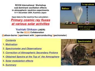
RCCN International Workshop sub-dominant oscillation effects in atmospheric neutrino experiments 9-11 December 2004, Kashiwa JapanInput data to the neutrino flux calculation :Primary cosmic ray fluxes at various solar activitiesYoshiaki Shikaze (JAERI)for the BESS Collaboration To high altitude Balloon BESS spectrometer to be lunched (Balloon-borne Experiment with Superconducting Spectrometer) Spectrometer RCCN International Workshop sub-dominant oscillation effects in atmospheric neutrino experiments 9-11 December 2004, Kashiwa JapanInput data to the neutrino flux calculation :Primary cosmic ray fluxes at various solar activitiesYoshiaki Shikaze (JAERI)for the BESS Collaboration Contents 1. Motivation 2. Spectrometer and Observations 3. Correction of Atmospheric Secondary Protons 4. Obtained Spectra at the Top of the Atmosphere 5. Solar modulation effects 6. Summary (Balloon-borne Experiment with Superconducting Spectrometer)
Climax neutron monitor & Sunspot number Solar minimum Solar maximum Motivation : Solar activity
Solar Modulation To understand the solar modulation, it is important to know time variation of low energy proton flux precisely. For the precise measurement by balloon experiment (at 5g/cm2), we must estimate the contamination of the atmospheric secondary protons, because as the energy decrease, secondary protons increase rapidly. To understand the solar modulation, it is important to know time variation of low energy proton flux precisely. Precise Low energy P flux Atmospheric secondary P Secondary-to-primary ratio of proton flux at air depth of 5g/cm2 (Estimation results in Papini et al.) Motivation : for low energy flux below 1GeV
To understand the solar modulation, it is important to know time variation of low energy proton flux precisely. For the precise measurement by balloon experiment (at 5g/cm2), we must estimate the contamination of the atmospheric secondary protons, because as the energy decrease, secondary protons increase rapidly. For the secondary estimation, we can measure the cosmic-ray data during ascending and descending periods and can use the data at different air depths for the tune of the secondary calculation (using transport equations; Papini et al.). secondary P estimation Ascent and descent data BESS-99,2000 … ascent data (Cutoff Rigidity~0.4GV) BESS-2001 … descent data (Cutoff Rigidity~4.2GV). The observed data below the cutoff is pure atmospheric secondary protons. Motivation : for low energy flux below 1GeV Solar Modulation To understand the solar modulation, it is important to know time variation of low energy proton flux precisely. For the precise measurement by balloon experiment (at 5g/cm2), we must estimate the contamination of the atmospheric secondary protons, because as the energy decrease, secondary protons increase rapidly. Precise Low energy P flux Atmospheric secondary P
BESS Spectrometer 4. PID by mass measurement Mass = ReZ(β-2 - 1)1/2 50ps TOF counter dE/dx, β Tracker (in B=1T) R = pc/Ze Proton selection β-band cut (after dE/dx-band cut) Features 1. Large Acceptance of 0.3m2Sr 2. Compact and Simple Cylindrical Structure ⇒ High statistics & Small systematic error 3. Uniform magnetic field of 1T
Summary of BESS-2000 Pressure ~1000 km L y n n L a k e ( BESS-97~2000,2002 Cutoff Rigidity~0.4GV) Live time~2.1h ( BESS-2001 Cutoff Rigidity~4.2GV) Live time~30.5h Altitude F t . S u m n e r Balloon Observations Flight Map of BESS
Secondary Primary (Secondary Only) Comparison of the calculation with observation Cutoff effect 2nd-p production processes • Evaporation • Recoil • Slowing down • Spallation • Interaction loss • Ionization energy loss 5.82g/cm2 BESS-2001 Observed data ( Abe et al. ) loss processes Total(=primary +secondary ; Papini et al.) Primary C Secondary (Papini et al.) D 11.9g/cm2 E F A B Correction of Atmospheric Secondary Protons Secondary proton calculation (Papini et al.) based on transport equations
Comparison of the calculation with observation Comparison of the calculation with observation Cutoff effect Cutoff effect 2nd-p production processes • Evaporation • Recoil • Slowing down • Spallation • Interaction loss • Ionization energy loss Total (This work) 5.82g/cm2 5.82g/cm2 BESS-2001 Observed data ( Abe et al. ) BESS-2001 Observed data ( Abe et al. ) loss processes Secondary (This work) Total(=primary +secondary; Papini et al.) Total(=primary +secondary ; Papini et al.) Primary Primary C Secondary (Papini et al.) Secondary (Papini et al.) D 11.9g/cm2 11.9g/cm2 E F A B Correction of Atmospheric Secondary Protons modified Secondary proton calculation (Papini et al.) based on transport equations Tune recoil generation functionto agree with the observed proton data. [BESS-2001 at Ft. Sumner (cutoff rigidity~4.2GV)]
Comparison of the calculation with observation Recoil proton generation function Cutoff effect Total (This work) 5.82g/cm2 Papini et al. BESS-2001 Observed data ( Abe et al. ) Our detectable energy range Secondary (This work) Total(=primary +secondary; Papini et al.) Primary This work Secondary (Papini et al.) 11.9g/cm2 Correction of Atmospheric Secondary Protons modified Secondary proton calculation (Papini et al.) based on transport equations Tune recoil generation functionto agree with the observed proton data. [BESS-2001 at Ft. Sumner (cutoff rigidity~4.2GV)]
Growth curve (Air depth dependence) of proton flux at Lynn Lake [Cutoff R~0.4GV] Estimation as Primary +Secondary Kinetic Energy region: 0.29-0.34(GeV) Kinetic Energy region: 0.63-0.73(GeV) This work This work Papini et al. Papini et al. Observed proton data (BESS-2000 ascent data at Lynn Lake) Observed proton data (BESS-2000 ascent data at Lynn Lake) Correction of Atmospheric Secondary Protons Start from floating level
Proton and Helium Spectra at the Top of the Atmosphere from 1997 to 2002
Proton and Helium Spectra at the Top of the Atmosphere from 1997 to 2002 Kinetic Energy per Nucleon
Kinetic Energy per Nucleon Kinetic Energy per Nucleon Proton and Helium Spectra at the Top of the Atmosphere from 1997 to 2002
Proton flux Proton flux Proton flux Proton flux Proton flux Proton flux Proton and Helium Spectra at the Top of the Atmosphere from 1997 to 2002
(He flux) x 1/10 (He flux) x 1/10 (He flux) x 1/10 (He flux) x 1/10 (He flux) x 1/10 (He flux) x 1/10 Proton and Helium Spectra at the Top of the Atmosphere from 1997 to 2002
(Ek+m)2 – m2 I(Ek,r1AU ) = I(Ek+φ,rb ) x (Ek+φ+m)2 - m2 (ref. Φ~500MV for BESS-97 in Myers et al. ) I(r) / p(r)2 = I(rb ) / p(rb )2, E(r) = E(rb ) - φ demodulate Φ~500MV P1 -P2 Interstellar Proton Flux =AβR BESS-97 proton Solar modulation effects on our obtained data Force Field Approximation (1 parameter; Modulation parameter φ) I(r) / p(r)2 = I(rb ) / p(rb )2, E(r) = E(rb ) - φ
(Ek+m)2 – m2 I(Ek,r1AU ) = I(Ek+φ,rb ) x (Ek+φ+m)2 - m2 P1 -P2 Interstellar Proton Flux =AβR obtained by fitting Solar modulation effects on our obtained data Force Field Approximation (1 parameter; Modulation parameter φ) (ref. Φ~500MV for BESS-97 in Myers et al. ) fitting for Φ
Summary • To understand the solar modulation, it is important to know • time variation of low energy proton flux precisely. • Low energy proton and helium spectra at a different solar activities • during a period of solar minimum, 1997, through post-maximum, 2002 • have been measured by BESS. • Their spectra at TOA were obtained • by using the calculation of atmospheric protons • revised to agree withthe observed protons at different air depths. • The obtained spectra were consistent with other experimental data of • cosmic-ray measurements. • From the check of the solar modulation effects, • Interstellar Proton spectrum was obtained • by assuming a)Force Field Approximation, b) φ=500MV for BESS-97 • and c)simple spectrum formula with 3 parameters.