Advanced Sparse Vector Methods in Fault Analysis of Power Systems
This lecture explores the application of sparse vector methods in analyzing faulted power systems. It covers concepts such as Thevenin equivalents for fault current calculations and emphasizes the importance of elimination trees and factorization paths in solving sparse linear equations. The lecture elaborates on the objectives of obtaining fault currents in electrical networks, introducing efficient techniques for handling sparse matrices. Practical examples guide the understanding of formulating and solving problems related to power system faults using advanced algorithms.

Advanced Sparse Vector Methods in Fault Analysis of Power Systems
E N D
Presentation Transcript
Sparse Vector Methods Lecture #13 EEE 574 Dr. Dan Tylavsky
Application: Consider faulted power systems. • This system is electrically equivalent to: • By superposition:
First system has 0.0 A. p.u. fault current, so the total fault current may be calculated using the second network. • To calculate fault current in second system we first represent the rest of the network as a Thevenin equivalent.
Once we have the Thevenin equivalent at a bus, we then calculate the fault current using the following network: • Assuming the network is linear, we find AN open circuit voltage (assuming all internal sources are deactivated) for A 1 p.u. current injection at the node of interest.
We can find the open circuit voltage by solving the equation:
Once we find the ZThevenin, we can then find the short circuit current due to prefault voltage VPreFault. Call that If. • We then want the currents flowing in branches near node, k, for instance.
To get these voltages we need to solve problems of the form: • X=don’t care values
Sometimes we wish to solve LUx=b when b is sparse and the elements we want to know in x are sparse. • When b and x are very sparse it is advantageous to use sparse vector methods. • Defn: Elimination Tree - A graph specifying the order in which rows of a matrix must be processed (during factorization or F/B substitution) if all precedence relationships are to be obeyed.
Theorem (Without Proof): All precedence relationships in LU factorization and F/B substitution will be obeyed if the nodes are ordered using the following algorithm: The node k must immediately precede node j if the lowest numbered below diagonal element in column k of L occurs in row j. (This is proved using the Fill-in Theorem.)
4 5 2 6 3 7 1 !!!!!!!!!!!!!!!!!!!!!!!!!!!!!!!!!!!!!!!!!!!!!!!!!!!!!!!!!!!!!!!!!!!!!L(U) Data structure requirements: The lowest-numbered, non-zero off diagonal element in each column of L (row of U) must be directly accessible without search (if efficiency is to be maintained.) * L(C), U(R), D, CO works. !!!!!!!!!!!!!!!!!!!!!!!!!!!!!!!!!!!!!!!!!!!!!!!!!!!!!!!!!!!!!!!!!!!!!!
Defn: Singleton - A vector with one non-zero element. • Defn: Factoriztion Path (Factor Path, or Path) - An ordered list of columns of L (rows of U) used in the solution of Lx=b. • Defn: Singleton Path - Factor Path for a singleton. • The factor path for a group of singletons may be found by appending to the front of each factor path the unique elements of the factor path of subsequent elements in the singleton list.
Example: Find the factor path for the singletons b={b1, b2}, for the matrix shown below. 2, • Factor path ={ 1,4,5,6,7}
Teams: Draw the elimination tree for the following L matrix from a factored A matrix and find the factor path for the singletons b={b4, b8}.
4 2 5 2 3 3 6 w 7 7 • Example: For the following matrix, find the value for x2, given that the only non-zero in the b vector is b3=2. 1 6 Fast Forward Factor path ={3,7} Fast Backward Factor path ={7,6,2}
Individually: For the following matrix, find the value for x8, given that the only non-zeros in the b vector are {b4, b8}={2,2}. (Process L by cols. U by rows.)
Example: Using a self-referential linked list construct the factor path for the U matrix shown if the b vector has non-zero’s in position 2 and 5. Step 1.1: Enter position of first non-zero as Initial Link Pointer and in switch array. Step 1.2: Use ECP and Rindx to find factor path and enter in switch array. Step 2.1: Compare next native b non-zero loc. w/ switch array and enter in link if new. Step 2.2: Use ECP and Rindx to find factor path and merge into Link.
Example: Using a self-referential linked list construct the factor path for the U matrix shown if the b vector has non-zero’s in position 2 and 5. Step 2.2: Use ECP and Rindx to find factor path and merge into Link. Result: Complete factor path is {5, 2, 6, 7}.
1 4 2 5 3 6 7 • Example: Perform fast forward (FF) substitution using the L/U matrix shown below if the b3=2, b5=1 (all other bi’s are zero). Factor Path = {5, 2, 6, 7}
Step 0: Zero B locations according to factor path. Step 1: Overwrite B locations according to non-zeros. Step 2.1: Perform Forward substitution by columns for 1st element in path. Step 2.2: Perform Forward substitution by columns for 2nd element in path. Step 2.3: Perform Forward substitution by columns for 3rd element in path. Step 2.4: Perform Forward substitution by columns for 4th element in path. (If this matrix has elements on the diagonal, then operate else finished.) Solution is {b2, b5, b6, b7}= {2, 1, -4, 18 } Perform Fast Backward substitution using appropriately ordered factor path if Ux=w is needed.
Results of using FF & FB: • Defn: (p:N N:k) as full (sparse) forward substitution starting with row/column p and full (sparse) backward substitution ending with row/column k. • Scenario: bk is known, xk is desired.
Defn: Neighborhood of length k about node m: The set of all nodes which can be reached by starting at node m and traversing at most k branches. Results show that getting solutions for nodes in a neighborhood of a node, k, requires only slightly more work than required for the solution of only node k.