Download
1 / 16
160 likes | 178 Vues
This tutorial explains the concept of maximum likelihood estimation (MLE) and its application in pattern recognition. It covers the general principle of MLE, its mathematical formulation, and its application in the case of Gaussian distributions. The tutorial also discusses the convergence of MLE estimates and the relationship between the MLE estimate and the true parameters.

E N D
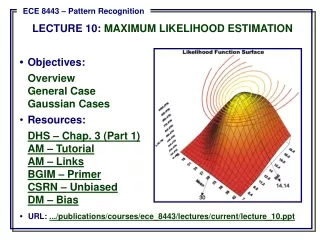
• Objectives: Overview General Case Gaussian Cases Resources: DHS – Chap. 3 (Part 1) AM – Tutorial AM – Links BGIM – Primer CSRN – Unbiased DM – Bias ECE 8443 – Pattern Recognition LECTURE 10: MAXIMUM LIKELIHOOD ESTIMATION • URL: .../publications/courses/ece_8443/lectures/current/lecture_10.ppt
10: MAXIMUM LIKELIHOOD ESTIMATION INTRODUCTION • In Chapter 2, we learned how to design an optimal classifier if we knew the prior probabilities, P(i), and class-conditional densities, p(x|i). • What can we do if we do not have this information? • What limitations do we face? • There are two common approaches to parameter estimation: maximum-likelihood and Bayesian estimation. • Maximum likelihood: treat the parameters as quantities whose values are fixed but unknown. • Bayes: treat the parameters as random variables having some known prior distribution. Observations of samples converts this to a posterior. • Bayesian learning: sharpen the a posteriori density causing it to peak near the true value.
10: MAXIMUM LIKELIHOOD ESTIMATION GENERAL PRINCIPLE • I.I.D.: c data sets, D1,...,Dc, where Dj drawn independently according to p(x|j). • Assume p(x|j) has a known parametric form and is completely determined by the parameter vector j (e.g., p(x|j) N(j,j), where j=[1, ..., j ,11, 12, ...,dd]) • p(x|j) has an explicit dependence on j:p(x|j,j) • Use training samples to estimate 1, 2,..., c • Functional independence: assume Di gives no useful information about j for ij • Simplifies notation to a set D of training samples (x1,...xn) drawn independently from p(x|) to estimate . • Because the samples were drawn independently:
The value of that maximizes this likelihood, denoted , is the maximum likelihood estimate (ML) of . 10: MAXIMUM LIKELIHOOD ESTIMATION EXAMPLE • p(D|) is called the likelihood of with respect to the data. • Given several training points • Top: candidate source distributions are shown • Which distribution is the ML estimate? • Middle: an estimate of the likelihood of the data as a function of (the mean) • Bottom: log likelihood
10: MAXIMUM LIKELIHOOD ESTIMATION GENERAL MATHEMATICS • The ML estimate is found by solving this equation: • The solution to this equation can be a global maximum, a local maximum, or even an inflection point. • Under what conditions is it a global maximum?
A class of estimators – maximum a posteriori (MAP) – maximize where describes the prior probability of different parameter values. 10: MAXIMUM LIKELIHOOD ESTIMATION MAXIMUM A POSTERIORI (MAP) • An ML estimator is a MAP estimator for uniform priors. • A MAP estimator finds the peak, or mode, of a posterior density. • MAP estimators are not transformation invariant (if we perform a nonlinear transformation of the input data, the estimator is no longer optimum in the new space). This observation will be useful later in the course.
because: which implies: 10: MAXIMUM LIKELIHOOD ESTIMATION GAUSSIAN CASE: UNKNOWN MEAN • Consider the case where only the mean, = , is unknown:
10: MAXIMUM LIKELIHOOD ESTIMATION GAUSSIAN CASE: UNKNOWN MEAN • Substituting into the expresssion for the total likelihood: • Rearranging terms: • Significance???
10: MAXIMUM LIKELIHOOD ESTIMATION UNKNOWN MEAN AND VARIANCE • Let = [,2]: • The full likelihood leads to:
The true covariance is the expected value of thematrix , which is a familiar result. 10: MAXIMUM LIKELIHOOD ESTIMATION UNKNOWN MEAN AND VARIANCE • This leads to these equations: • In the multivariate case:
10: MAXIMUM LIKELIHOOD ESTIMATION CONVERGENCE OF THE MEAN • Does the maximum likelihood estimate of the variance converge to the true value of the variance? Let’s start with a few simple results we will need later. • Expected value of the ML estimate of the mean:
which implies: 10: MAXIMUM LIKELIHOOD ESTIMATION VARIANCE OF ML ESTIMATE OF THE MEAN • The expected value of xixj will be 2 for j k since the two random variables are independent. • The expected value of xi2 will be 2 + 2. • Hence, in the summation above, we have n2-n terms with expected value 2 and n terms with expected value 2 + 2. • Thus, • We see that the variance of the estimate goes to zero as n goes to infinity, and our estimate converges to the true estimate (error goes to zero).
Note that this implies: 10: MAXIMUM LIKELIHOOD ESTIMATION VARIANCE RELATIONSHIPS • We will need one more result: • Now we can combine these results. Recall our expression for the ML estimate of the variance:
10: MAXIMUM LIKELIHOOD ESTIMATION COVARIANCE EXPANSION • Expand the covariance and simplify: • One more intermediate term to derive:
10: MAXIMUM LIKELIHOOD ESTIMATION BIASED VARIANCE ESTIMATE • Substitute our previously derived expression for the second term:
10: MAXIMUM LIKELIHOOD ESTIMATION EXPECTATION SIMPLIFICATION • Therefore, the ML estimate is biased: However, the ML estimate converges (and is MSE). • An unbiased estimator is: • These are related by: which is asymptotically unbiased. See Burl, AJWills and AWM for excellent examples and explanations of the details of this derivation.