Transverse Beam Dynamics Part 2
Transverse Beam Dynamics Part 2. Piotr Skowronski In large majority based on slides of O.Brüning http://bruening.web.cern.ch/bruening/ and http ://cds.cern.ch/record/941313?ln=en B.Holzer https:// indico.cern.ch/event/173359/contribution/9/material/0/0.pdf

Transverse Beam Dynamics Part 2
E N D
Presentation Transcript
Transverse Beam DynamicsPart 2 Piotr Skowronski In large majority based on slides of O.Brüning http://bruening.web.cern.ch/bruening/ and http://cds.cern.ch/record/941313?ln=en B.Holzerhttps://indico.cern.ch/event/173359/contribution/9/material/0/0.pdf W.Herrhttp://zwe.home.cern.ch/zwe/ Y.Papaphilippouhttp://yannis.web.cern.ch/yannis/teaching/ B. Goddard
Overview • Next in transverse beam dynamics to follow • Errors from different kinds of elements • Orbit correction • Decoherence • Filamentation • Amplitude detuning • Resonances • Tune diagram • Dynamic aperture • Coupling
Exercise 1 • Simulate motion of a particle with some initial x and px around a ring • Plot the coordinates every turn for 50k turns • Assume different phase advance and observe how the particle moves. In particular when tune is close to • 1 • 0.5 • 0.333 • Put 10 particles with different amplitudes • Add a small dipole error. Normally magnets are within 1e-4. • Bring the tune towards integer
Integer resonance • Dipole kicks add up • A smallest dipole errormake the particles driftaway
Exercise 1 • Move away from integer to 0.5 • Add quadrupole error and choose a random not round tune • Bring tune close to 0.5
Half-integer tune • Dipole errors are nicely damped • But quadrupole errors add-up
Exercise 1 • Add sextupole kick and see what happens around 1/3 tune • Octupole and close to 0.25 • Why the tune needs to be little bit less to observe the features? • Amplitude detuning
Exercise 2 • Add the second plane, implement a sextupole kick • Keep some sextupole and choose tunes 0.18 and 0.62 • Bring the vertical tune towards 0.59 • Why do you see the “features”? What is the condition for a resonance?
Saturn • The gaps between rings are due to resonances
Resonance condition • Tune diagram:
Error Sources • Linear field errors • Magnetic field imperfections from design values • Powering errors • Feed-down errors due to transverse alignment errors or bad orbit (regular precision: ± 0.1 mm) • Roll positioning errors (creates coupling) (± 0.5 mrad) • Beam energy errors (change of normalized strength) • Calibration • Non-linear field errors • Naturally it is impossible to build a perfect magnet
Accelerator sensitivity • Off-center magnets change the beam optics • Dispersion and focusing • Usually not possible to correct entirely • It spoils emittance and luminosity • Alignment • Vibrations and ground motion
Accelerator sensitivity LEP: When people sleepthe machine is stable
Accelerator sensitivity LEP: Trains changed the bending magnet field
LEP sensitivity • LEP energy (green dots) andexpected effect due to two-bodymotion of the moon and the earth • Below LEP energy and orbitchange with the lake water level
Accelerator sensitivity • Magnet motion in HERA, Hamburg
Accelerator Sensitivity • LEP beam felt moon position (tides) and the lake water level • Linear Colliders with their nano-meter emittance care about nano-meter ground motion • For example, Atlantic haul is sensible in Geneva at this level • Need active stabilization • Beam based alignment
Feed-down errors • Example of a quadrupole • If beam orbit passes off center at xm • then B field is • Beam sees it as dipole plus quadrupole • is constant, hence gives a constant kick • Combined function magnet is a largely displaced quad • The same way an off-center sextupolecreates extra focusing
Skew Multipoles Example: Skew Quadrupole • Quadrupole rotated by 45° gives a skew quadrupole • Horizontal kick depends on vertical offset
Errors TreatmentPerturbed Hills equation • The force term is the Lorenz force of a charged particle in a magnetic field: • Where q is x or y • w0: constant b-function and phase advance along the storage ring • F is arbitrary function of all coordinates • Generally this equations are not solvable • Need a numerical integration • Some special cases can be solved • They eventually give some insight into specific effects
Errors TreatmentPerturbed Hills equation • To simplify we normalize the coordinates • It converts the ellipse into a ring • frequency becomes independent of s: • The force term is the Lorenz force of a charged particle in a magnetic field: • Where q is x or y • w0: constant b-function and phase advance along the storage ring
Errors to linear motion • Perturbation from a dipole filed error • Perturbation from a quadrupole filed error • Using the normalized multipole strengths
Multipole Expansion of Magnetic Fields Taylor expansion of the magnetic field: with multipole order Bx By dipole 0 quadrupole 1 sextupole 2 octupole 3 skew multipoles an: rotation of the magnetic field 90o for dipole magnets by half of the coil symmetry:45o for quadrupole magnets 30ofor sextupole magnets 23
Perturbed Hills Equation perturbed equations of motion: By Bx normalized multipole gradients : with: 24
Perturbed Hills Equation • General solution of this type of equations is linear combination of • Solution of homogenous equation where F is set to 0 • Particular up solution that we usually guess, for example • F=cos(x) up=apcos(x) • F=x3 up=ap3x3 + ap2x2 + ap1x + ap0 • Perturbation theory • Calculate recursively corrections to higher and higher orders hoping that few terms will be sufficient to find an accurate solution • Does not really work • For example breaks in vicinity of resonances • Does not reveal all the details of the dynamics • Still, some features can be studied • The proper way to proceed is the normal form analysis • It is quite vast and heavy topic, I spare it for a separate lecture
Perturbation theory vs tracking • 1st order perturbation theory
Perturbed Hills Equation perturbed equations of motion: The RHS can be Fourier decomposed Homogenous solution Particular solution By substituting we find Fourier coefficients of the particular solution Any of them can diverge if Resonances!
Dipole error • The orbit can be treated as a single particle • It obeys • At s0, after one turn, it receives additional kick x’(s0) = Δk0 • The kicked orbit must close on itself after one turn
Dipole error: perturbed orbit • These coordinates can be propagated to arbitrary point using transfer matrix • It is symmetric around the error position • If Q is an integer then closed orbit does not exist! Orbit ‘kink’ for single perturbation (SPS with 90o Q = n.62): 29
Quad error • A focusing error can be represented as additional thin lens quadrupole strength • Where is unperturbed map • Modified one turn map is
Quad error: tune change • For distributed errors we have to integrate around ring • As bigger the beta function as more the error prenounced • Biggest errors from final focus quadrupoles
Quad error: β-function change • Recall general solution Hills equation is linear combination of sine like and cosine like • Assume error at position s0 • Transfer map is also modified by the error • One turn map at the start can be transformed to an arbitrary position s as • Since the error is at s0 so is not affected = =
Quad error: β-function changeArithmetic for reference • Inserting • We get • Use and = =
Beta-function error • Keeping 1st order in • And for the all errors in the ring • Beta function error is oscillatory (Beta beat) of twice the betatron frequency • Errors around the ring average out due to different phases • Use all the quads for tune correction, it will affect beta less • Or use 2 quads with the same beta but 90 degree apart • Tune will change, but beta changes will cancel
Natural Chromaticity • Offset in particle energy can be seen as offset in focusing strength • The resulting tune changeis natural chromaticity • Chroma without sextupole correction
Chromaticity • Off centre sextupole • Using dispersion orbit we get focusing change • And resulting chromaticity • Chroma correction strength is proportional to • Beta inside the sextupole • Dispersion • Strength of the sextupole
Orbit Correction • Deflection angle: • Trajectory response: • Closed orbit bump • compensate the trajectory response with additional dipole fields further down-stream ‘closure’ of the perturbation within one turn
2 corrector bump • In case of an orbit error it is the best to correct it at the place • Requires a corrector at every element • Eventually, we can try to correct after π phase advance • Limits: • Must be lucky to find a corrector exactly after π • Sensitive to BPM errors • Large number of correctors
3 corrector bump • Closure • Works for any type of lattice • Limits: • Sensitive to BPM errors; • Need large number of correctors
4 corrector bump • Of course one can involve any number of correctors
Global correction • A is orbit response matrix on correctors excitation • n x m matrix • n BPMs • m corrector magnets • Can be obtained from the machine model • Or measured • Excite each corrector and observe orbit change • We can write the orbit as • Correction is • Problem: A is normally not invertible • It is normally not even a square matrix! • Solution: minimize the norm
SVD Algorithm • Find a matrix B such that • Attains a minimum with B being a m x n matrix and: • Singular value decomposition (SVD): • Any matrix can be written as: • where O1 and O2 are orthogonal matrices and D is diagonal • D has diagonal form • Define a pseudo inversematrix • 1k being the k x k unit matrix
SVD Algorithm • Correction matrix defined as • Main properties • SVD allows you to adjust k corrector magnets • If k = m = n one obtains a zero orbit (using all correctors) • For m = n, SVD minimizes the norm (using all correctors) • The algorithm is not stable if D has small Eigenvalues • Can be used to find redundant correctors! • Nota bene, SVD is extensively used to clean the measured data and hence reduce errors of the measurements
Most effective corrector • the orbit error is dominated by a few large perturbations: • minimize the norm:using only a small set of corrector magnets • brut force: select all possible corrector combinations • time consuming but god result • selective: use one corrector at the time + keep most effective • much faster but has a finite chance to miss best solution and can generate p bumps • MICADO: selective + cross correlation between orbit • residues and remaining correcotr magnets
LEP • See the phase advance…
Harmonic Filtering • Unperturbed solution (smooth approximation): • In case of orbit perturbation • F and Closed Orbit are periodic Fourier decomposition • Closed Orbit Fourier peak around tune • Distribute correctors to filter out the main harmonics
Matching ring injection • Ring has a unique closed solution in terms of orbit and Twiss parameters • What happens if beam injected not onto this solution? • If beam was perfectly monochromatic orthere was no chromaticity or amplitude detuning the beam was beat around the closed solution • But real bunches and real accelerators are never perfect:decoherence and filamentation
Decoherence • Effect of the orbit error