System Modeling
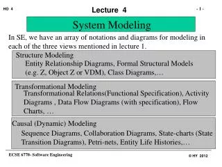
System Modeling. In SE, we have an array of notations and diagrams for modeling in each of the three views mentioned in lecture 1. Structure Modeling. Entity Relationship Diagrams, Formal Structural Models (e.g. Z, Object Z or VDM), Class Diagrams,…. Transformational Modeling.

System Modeling
E N D
Presentation Transcript
System Modeling In SE, we have an array of notations and diagrams for modeling in each of the three views mentioned in lecture 1. Structure Modeling Entity Relationship Diagrams, Formal Structural Models (e.g. Z, Object Z or VDM), Class Diagrams,… Transformational Modeling Transformational Relations(Functional Specification), Activity Diagrams , Data Flow Diagrams (with specification), Flow Charts, … Causal (Dynamic) Modeling Sequence Diagrams, Collaboration Diagrams, State-charts (State Transition Diagrams), Petri-nets, Entity Life Histories,…
Structure Modeling • Structure modeling is modeling of things and their situational relationships. A photograph is a good structure model. It shows things that were there when the picture was taken and how they were situated with respect to one another. • We can similarly compose diagrams or other models of a problem situation in which we depict all the relevant things and relationships. • There are many ways to do this. We shall discuss the three most popular and prevalent of these. Namely: • Entity Relationship Modeling which is used mainly for database design • Formal Schemas and Formal Object Schemas (using Z and Object Z) • Class Diagrams (using UML) used mainly as part of object oriented modeling
Structure Modeling Entity Relationship (ER) Modeling: This is an informal (or semi-formal) approach to structure modeling in which a situation is studied so that static and persistent elements in it are identified, along with their static relationships. A collection of like elements is called an entity. A mapping of elements of one entity onto another entity (or itself) is called a relationship. Entities are defined in terms of a name and a set of attributes. Relationships are defined in terms of a verb phrase (e.g. works-for) that establishes the nature of the mapping between the entities. The results of ER modeling are almost always shown using diagrams. There are many different conventions. In the absence of an industry standard, we use a popular one here of my preference.
Structure Modeling Example: Department Employee Name: Location: Budget: m Works-For 1 Name: SSN: Salary: This means that there are many elements belonging to the set Employee (i.e. many persons employed) each is mapped into (has a relationship with) only one element belonging to the entity Department (a specific department). The relationship is that this particular employee works for one specific department. For each employee we keep his or her name, social security number and current salary. For each department we keep the name of the department, its location and its budget. You will learn (or may have already learned) a lot more about this modeling approach in your database course.
Structure Modeling Formal Object Schemas: Object Z Stack[T] max:N items: seq T #items max INIT items =‹ › Push ( items) item?:T #items < max items’ = ‹item?›⁀items
Structure Modeling Pop ( items) item!:T item! ‹ › items = ‹item!›⁀items’ top ( items) item!:T item! ‹ › items’ = items
Causal Modeling • There are many different approaches to causal modeling. Whilst they all attempt to do the same thing, they are not all of the same level of capability, formality, ease of use or learnability. In this course we cover a number of popular approaches to causal modeling, including: • Entity Life Histories • The UML suite of dynamic modeling facilities, which include • Petri-nets Sequence diagrams Collaboration diagrams State diagrams
Causal Modeling Entity Life Histories These are diagrams that depict the various states of a class or type of object from inception to demise. Usually used in relation to persistent database “entities”, they can become overwhelmed if the states are too numerous or the object can possess concurrent states. They also do not necessarily depict the events that lead to state transitions. EMP ARCHIVE UPDATE RETIRE REPORT INIT CREATE * *
Causal Modeling Petri nets: Petri nets are a formal graphical approach to causal modeling. They improve on the capabilities of state diagrams by allowing for proper description of some major issues in concurrency such as synchronization, deadlocks and conflicts. Petri nets are composed of two types of nodes and one type of arc. The two types of node are called places and transitions. The arc is called an event. A fourth artifact called a token, when located inside a place, marks it as enabled.
Causal Modeling A Petri net composed of five places P={p1,p2,p3,p4,p5} and three transitions T={t1,t2,t3} p1 t1 p2 p3 A token ( ) inside a place indicates that the place has satisfied all pre-conditions for causing an event to occur. Such a place is called “enabled” t2 p5 p4 A transition takes place only when all places leading to it are enabled. Such a transition is called an enabled transition. t3
p1 A transition takes place to p2. But t2 is not enabled as p3 is not enabled. t1 p2 p3 t2 p5 p4 t3 Causal Modeling P1 is enabled, thus enabling t1 The system stops here.
p1 t1 p2 p3 t2 p5 p4 t3 Causal Modeling
Causal Modeling p1 p’1 t1 t’1 p2 p3 p’2 p’3 t2 t’2 p5 p4 p’4 ? t3 t’3 Conflict
Causal Modeling p1 t1 p2 p3 p5 t2 ? p4 t3 Deadlock
Transformational Modeling Transformation modeling is the third modeling view. It answers the question “how”. Depending on level of granularity there are many techniques. Including: Abstraction Level: Dataflow Diagrams Activity Diagrams Low Level: Pseudo-code Flowcharts etc. Not part of UML
Transformational Modeling Flow charts Flow charts depict the flow of control. They show how operations are performed and decisions made by depicting how the control in the program is exchanged from the beginning to the end of all paths of interest. Flow charts show how the program works. Flow charts are composed of a number of node types and one type of arc. The node types are: Start/End node Transformation node Decision node Link node Special processing nodes Logic nodes
Transformational Modeling Flow charts can be high level or low level High level flow charts depict the flow of control at a high level of granularity, such as the organization or the entire system. Low level ones usually depict the flow of control in a specific program unit. The difference between a high level and low level flow chart is that in a low level flow chart all transformational nodes contain transformations that can not be usefully broken down to simpler flowcharts themselves. By this we mean doing so would produce transformation at a lower level of granularity than that of the target programming language.
Transformational Modeling Flow chart nodes: Start/End nodes: These mark the beginning and end of a flow within a flowchart Terminator Transformation nodes: These show a logical step taken Transformation Alternate transformation Manual transformation
Transformational Modeling Decision nodes: These show alternate conditions or paths the flow may take Condition Logic nodes: These are logical operators such as AND, OR and NOT NOT AND OR Link nodes: These connect various parts of the diagram (e.g. continue on next page) Off page connector On page connector
Transformational Modeling Special processing nodes: These are nodes that depict specific large scale processing or machine interaction. Useful in the early days when flowcharting was amongst the only modeling methods available, they are now largely disused. Punched card Manual input Other mag. storage Stored data Punched tape Disk Delay Console or display Seq. Access device Extract Merge Collate Internal storage Sort
Transformational Modeling Start A=A+B N=N-1 Read N F N=0 F N>0 T T Write A Read A,B End
Transformational Modeling Data Flow Diagrams Data flow diagrams depict the flow of data. They show how data received as input is changed to outputs by the various operations performed. Data flow diagrams show how the data changes. Basic data flow diagrams are composed of a number of node types and one type of arch. The node types are: External Entities (Sources and Sinks) Processing node Data-stores Link nodes
Transformational Modeling External entities (sources and Sinks): These are entities outside the scope of our focus that provide the inputs from the outside or receive the outputs generated. They are labeled by a noun or an object or class name. Customer Process nodes: These depict the processing that is done to the inputs into that process to form the output. Usually these nodes are labeled by a verb phrase representing the nature of the processing to be done and a number sequence depicting the process and its level 1.4.7 1.4.7 Book seat Book seat
Transformational Modeling Data-stores: These are buffers where interim outputs generated are stored for future usage. Data-stores are usually named. Primary Buffer Link nodes: They connect the various parts of the diagrams to yield a less cluttered result. They are usually numbered or carry a symbol. 22 The only arc is called a dataflow and it depicts the flow of data (as input into or output from) an external entity or process. They are usually named. client address
Transformational Modeling Market Stock Price Invalid Req. Advice 1.2.2 Prepare SX Transaction Sell Advice 1.2.1 Validate Sell Sell Validation No. of Stock owned Account 1.2.3 RegisterTransaction Account Sell Example DFD Account Update Transaction Advice Sell Details Trans. Confirmation Sell Stock; Level 3
Transformational Modeling Data Flow diagrams may depict a situation at multiple levels of granularity. By that we mean a process in a data flow diagram may be decomposed into an entire new dataflow diagram at a lower level, and so on. At each lower level, there will be more detail of the model visible. Conversely, one can say that a higher level process can be described in terms of a dataflow diagram composed of simpler, lower level processes, data flows and data-stores. However this decomposition process must stop at some stage. At that stage we shall still have a dataflow diagram that only depicts the transformation of inputs to outputs of various processes. It however does not say HOW each leaf level process should achieve this. This may be obvious but is not defined.
Transformational Modeling Important Note: Dataflow diagrams are more so a mechanism for abstraction than a transformational modeling technique. They must be accompanied by a complementary mechanism that defines the leaf level transformations. Something like a flowchart of each leaf process, a pseudo-code, mathematical equation, truth table or formal definition is needed.
Transformational Modeling Pseudo-code: begin Read r,a; Declare x,y; if { (a) L.T. 0 a=(-1)*a; }; Set x to r*sin(a); Set y to r*cos(a); Write x; Write y; end 1.5.6 x r Convert to Cartesian y a
Transformational Modeling Mathematical expression: 1.5.6 Desc. For 1.5.6 x r Convert to Cartesian y a
Transformational Modeling ACTIVITY DIAGRAMS Activity diagrams depict the processing aspects of the system. They are similar to flowcharts except: Activity charts allow synchronization They are similar to dataflow diagrams except: Transition between activities is via conditions not data. Activity charts allow synchronization
Transformational Modeling Stock Manager Order Processing Finance Receive Order *[for each line item on order] Select Outstanding order item Receive Supply [notify supply] Check Line Item * [for each chosen order item] Check order Assign Goods to Order [failed] [succeeded] [out of stock] [in stock] Assign Item to Order Cancel Order Authorize payment Reorder Item Add Remainder to Stock Dispatch Order [all outstanding order items filled] [Stock assigned to all line items and payment authorized]
Structure Transformation Causality Objects Classes Relationships Inputs Outputs Transformations Events States Sequences ENCAPSULATION
UML has a an array of notations and diagrams for modeling in each of these three views. Structure Modeling Class notation, object notation, Associations, Links, Class diagrams, object diagrams,… Transformational Modeling Actors, Transformational relations, Use Case diagrams, Context Diagrams, Activity diagrams ,Transformational definitions, …
Causal (Dynamic) Modeling Events, Activities, Actions, Transitions, States, Sequence diagrams, Collaboration diagrams, Statechart diagrams, etc.… In the next session we shall start with structural modeling and introduce some important elements of the UML notation set.
Objects Classes Associations Links Structural Modeling: Answers the question WHAT? Class Diagram We need to concentrate on static relationships between objects (SNAPSHOT). So, we need to depict:
CLASSES The implementation of a type A generator for instances A class is depicted as a solid-outlined rectangle with compartments: • Must have a name compartment • May have other compartments (up to 3 more)
Name Compartment Attributes Compartment Operations Compartment Other Compartment The other compartments may contain: Compartment 2: Attributes Compartment 3: Operations Compartment 4: Others (Business rules, exceptions, etc.) Widget color: Color position:Coord=(0,0) move(from:Coord,to:Coord=(50,50)) get_color( ):Color draw( ) draw_all( ) color /= “white”
Class name and the class name compartment: • The name compartment must be present • The name compartment contains the name of the class. Class names are centered, begin with a capital letter and are in boldface. Abstract class names are italicized.
Attributes and the attribute compartment: • May be omitted when drawing high level diagrams • Are denoted as left justified plain lowercase text strings • The name may be followed by a colon ( : ) followed by the type of the attribute • Optionally we can set the initial value of the attribute. To do so, the type name is followed by ( = ) and then the value
May contain a visibility tag. A visibility tag could be: • + Public • # Protected • - Private
Operations and the operations compartment: • May be omitted when drawing high level diagrams • Are denoted as left justified plain lowercase text strings. Abstract operations are italicized • May have parentheses containing a comma separated list of the parameters of the method that implements the operation. • Optionally the parameter list may have indicators. These are:
in Parameter is only passed in to the operation out Parameter is only passed out (returned) inout Both (Default is “in”) • May have a return list containing one or a comma separated list of more than one formal parameters following a colon after the parameter list. • Multiple return parameters, if there, must have a name and a type separated by a colon.
An operation may have a class scope. Class operations are underlined. • May contain a visibility tag. A visibility tag could be: • + Public • # Protected • - Private
Usually we do not bother with this level of detail unless we aim to generate code automatically Attribute - color:Color=red Operation: # credit_rating(in candidate:Customer=current, in agency: Agent=dandb) : rating : Integer, reason : Text
TEMPLATES AND GENERIC CLASSES T1,T2 PAIR first:T1 second:T2 Pair <Integer, Integer> OR set_first(in T1) set_second(in T2) out( ): STRING <<bind>> (Integer,Integer) Pair
OBJECTS An element of a type set. An instance of a class. An object is depicted as a solid-outline rectangle with up to 3 compartments: • The top compartment is the name compartment. • May have other compartments (up to 2 more)
Name Compartment Attributes Compartment Other Compartment The other compartments may contain: Compartment 2: Attribute values Compartment 3: Other doowak: Widget color=Red position=(10,45)
Object name and the name compartment: • The name compartment must be present • The name compartment contains the name of the object; if a name exists. The name structure, if there, must be underlined. If the name is not there, or for “un-named” objects, the colon must remain. • The name may be followed by a colon ( : ) followed by a comma separated list of class to which the object belongs.
:Widget color=Red position=(10,45) : An un-known or un-named object An object, any object
Attribute values and the attribute values compartment: • It is optional and may not be present. • If present, it contains the names of the relevant attributes of the class of which this object is an instance and the values relating to that attribute. • Only attribute names and values of interest should be shown.