Download
1 / 50
500 likes | 674 Vues
From Experiments to Closed Loop Control II: The X-files. Håkan Hjalmarsson Department of Signals, Sensors and Systems Royal Institute of Technology. Controller. The Problem. Outline. Feedback. G 0. Noise. Exp. constraints. Perf. specs. Open loop/ Closed loop. Robust control. max.

E N D
From Experiments to Closed Loop Control II: The X-files Håkan Hjalmarsson Department of Signals, Sensors and Systems Royal Institute of Technology
Controller The Problem
Outline Feedback G0 Noise Exp. constraints Perf. specs Open loop/ Closed loop Robust control max C(G) G0 Spectra Validatoin Experiment Experiment design C(G) Inform. contents min Parameter estimation max max max max max G +D - Prior information • True system acts as disturbance Model complexity min min min min min Performance specifications Computational resources User skill ”Feedback” beneficial !! • Control design/Estimator=Controller
Robust Control • Frequency by frequency bounds on the model error usually required for robust stability and robust performance • Trade-off performance vs model quality, e.g: • |D| = |(G0 G -1 - I ) T(G,C)| • sufficiently small
Next Topic: Parameter Estimation Feedback G0 Noise Exp. constraints Perf. specs Open loop/ Closed loop Robust control max C(G) G0 Spectra Experiment Validatoin Experiment design C(G) Inform. contents min Parameter estimation max max max max max G +D - Prior information What are the means to control the model error in parameter estimation? Model complexity min min min min min Performance specifications Computational resources User skill
Parameter Estimation Essentials e0 (white noise, variance s2) H0= C0/D0 v G0 y G0= B0/A0 Parameter estimate: Limit estimate: True system: u Model: y = G(q)u + H(q)v,q2Rm Prediction error: e(q) = H(q)-1 (y- G(q)u )
Decomposing the Model Error Parameter estimation Limit model ^ ^ Model error: E [| G0 - G |2]= | G0 - G* |2 + E [| G * - G |2] MSE Bias Error Variance Error
The Bias Error Parameter estimation ) Can only tune the L2 norm of the bias error ) Cannot guarantee stability Much effort in literature on tuning the bias – Neglects information contents in data
Parameter estimation Statistical Aspects of Restricted Complexity Modeling Full order model Full order controller Model Reduced order model How should we identify a restricted complexity model such that noise impact minimized? Example: Data + Priors Reduced order controller Which way is best wrt statistical accuracy?
An Illustrative Example Restricted Complexity Modeling Statistical Aspects Estimate static gain: • The noise is white, Gaussian and has unit variance • Many parameters but
Restricted Complexity Modeling Statistical Aspects Full order model: Only one parameter: Variancecontribution from unmodeled dynamics Bias error Method 1: Maximum Likelihood (= Least-Squares) Method 2: Biased Biased beats ML!!
Restricted Complexity Modeling Statistical Aspects Bias error Variance of first parameter But ...... Why not take the first parameter of the ML estimate as estimate? • Same bias as biased estimate • Lower variance – no unmodelled dynamics that contribute ML beats biased!!
A Separation Principle Restricted Complexity Modeling Statistical Aspects AML of q AML of f(q) ^ ^ f(q) q The invariance principle in statistics:
Optimal Identification for Performance Restricted Complexity Modeling Statistical Aspects 1. Estimate ML model GML of G0 ) The minimizing G is a function of G0 2. Optimal reduced order estimate: Bonus: Stability can be checked
Restricted Complexity Modeling Statistical Aspects The Separation Principle Applications: • Model reduction (Tjärnström and Ljung) • Simulation (Zhu and van den Bosch) • Estimation of model uncertainty • I4C Conclusion: Always model as well as possible before any model simplifications
Summary Full order model Full order controller Reduced order model Restricted Complexity Modeling Statistical Aspects • For a given data set, always model as well as possible in order to ensure best possible statistical properties Data + Priors Reduced order controller
Restricted Complexity Modeling Moving Towards Real Applications • We have to accept that reality is always more complex than our models • Bias error in general not quantifiable frequency by frequency (unless priors are introduced) • How do we cope with this? • (and we do – there are numerous success stories)
Near Optimal Modeling Restricted Complexity Modeling Suppose Example continued: )One parameter model optimal (for estimating G(0) ) regardless of system complexity! Restricted complexity model same accuracy as ML!
Restricted Complexity Modeling Near Optimal Modeling
Non-singular Case Restricted Complexity Modeling Near Optimal Modeling Level set of åe2(t,q) • All models in confidence region qualify as good models (within a factor 2)! • LS-estimation provides near optimal models if MSE is small enough
Conclusions from Example Restricted Complexity Modeling Near Optimal Modeling • Experimental conditions can be used to: • Ensure near statistical optimality of restricted complexity models by making uncertainty large in certain ”directions” (Let sleeping dogs lie) • Allows the bias error to be assessed by the variance error 2. Ensure that certain system properties can be estimated accurately no matter the system complexity by making uncertainty small in certain ”directions”
The role of the noise model ^ |G±-G| Restricted Complexity Modeling Statistical Aspects Near Optimal Modeling Models with small MSE good ) Also noise model important Example: 3rd order Box-Jenkins system 2nd order OE 2nd order BJ 3rd order BJ Noise model useful in near optimal modeling!
Near optimal models and the separation princple ^ qN ^ hN Restricted Complexity Modeling Statistical Aspects Near Optimal Modeling f(q) Using near optimal estimates in the separation principle leads to near optimal estimates of h!
Summary Restricted Complexity Modeling Near Optimal Modeling • Models inside confidence region of full-order model are near optimal • Can be obtained by least-squares identification • The noise model is important • The separation principle is applicable • Experimental conditions determine which models are near optimal! • But we need full-order model for model error quantification - The Achilles heel.
Safe System Id Ensure that certain system properties can be estimated accurately no matter the system complexity by making uncertainty small in certain ”directions” How and for which system properties can this be achieved????? • Let’s examine the variance error! • and then experiment design issues
The Objective Safe System Id qno true parameters (n = dimension) hm=fn(qn) quantities of interest (e.g. nmp zeros, freq resp at certain freq. ....). Dimenson m<n. P=Covariance of qn Cov(hm) = fn´(qno)P[fn´(qno)]T Criterion: J=Trace(Cov(hm)) Constraint: sFu(w)dw·a Q: When can we choose Fu such that J is small regardless of n?
Some first insight Safe System Id Cov(hm) = fn´(qno)P[fn´(qno)]T Criterion: J=Trace(Cov(hm)) Constraint: sFu(w)dw·a Suppose fn´ normalized so that it is an ON-matrix Choose Fu such that “smallest” eigenvectors of P , fn´ This gives J= sum of m smallest eigenvalues of P (which are related to Fu)
FIR case Safe System Id • P-1= s-pp YnYn*Fu dw / l • where Yn=[1 e-jw ... e-j(n-1)w]T • Eigenvalue(P-1)=1/Eigenvalue(P) • P-1 and P have the same eigenvectors • Asymptotic results for P-1 (Grenander Szegö): • eigenvalues ,Fu(2p k/n), k=1,..n • eigenvectors ,Yn(2p k/n) (which are orthogonal)
Example Safe System Id
Safe System Id Eigenvalues of P vs Fu Cosine for angle between Yn and eigenvectors of P
Input Design Recipe Safe System Id • Choose freq for which Yn span fn´ • Choose Fu as large as possible at these freq. bins. How to combat system complexity: If Yn continues to span fn’ as n is increased, then the accuracy is insensitive to the model order cf static gain example!
Illustrations Safe System Id • NMP-zero estimates • Variance of frequency function estimates
NMP-zeros Safe System Id f’n=[1 zo-1 zo-2 ....]T • Tail elements become smaller and smaller • ) Variance converges as n!1
NMP zero MP zero Unit circle Safe System Id NMP-zeros Example Zero estimates for 50 realizations
The Variance Error of Frequency Funtion Estimates Covariance matrix of parameter estimate Safe System Id • Generally very complicated function of • Input spectrum Fu • Noise spectrum Fv • True system G0 • But can always be expressed as kn,N/ N Fv/ Fu • n = # estimated parameters
An archetypical variance expression Expression for ??? Variance of Frequency Function Estimates
Large sample expression (LSE) Variance of Frequency Function Estimates Asymptotic Expressions • Xie & Ljung (TAC 2001): Fixed denominator + AR input • Ninness and Hjalmarsson (TAC 2004): BJ model + AR input
Comparison with true variance Variance of Frequency Function Estimates Asymptotic Expressions TRUE LSE HOE-85
Safe System Id: FIR systems Safe System Id Variance of Frequency Function Estimates AR-input: u=1/F w, n=degree of F. Suppose x1¼ ejw1and all other poles at origin: • Last term dominates for w¼w1: Insensitive to model order • Last term small for w¹w1 : Variance grows linearly with order
Summary Safe System Id Variance of Frequency Function Estimates • Focusing the input spectrum to a certain frequency region makes the model accuracy less dependent on the model complexity in this range • Penalty at other frequency regions • Classical m/N Fv/Fu expression toooo optimistic variance approximation around narrow peaks of the input spectrum
Near Optimal Modeling Safe System Id Suppose I practice safe system id. Then I know that with a full order, or overparameterized, model I will get what I want. Q: What if I use a restricted complexity model? Well, for a near optimal model it has to be inside the confidence region of the full order model which means that it has to model the important system features accurately! cf static gain example!
Summary Safe System Id Modeling Paradigm: • Use input to reveal important system features • and be prepared to model these • ”Standard” model uncertainty estimates valid for these features • Let sleeping dogs lie • Ensure that application take large model uncertainties into account for other system features (the dogs) Make sure the data speaks what you need to hear!
Experiment Design for Safe System Id • Robust stability • NMP-zeros • One impulse response coefficient • (Static gain)
Experiment Design for Robust Stability Experiment Design Robust stability: Confidence bounds: Variance: Can be transformed into a problem that is convex in the autocovariances of the input, cf Märta’s talk on Monday Safe System Id: Design for higher system order than you believe the system to be
Experiment Design Input Design for Estimation of NMP-zeros MinFu E u2 s.t Var zNMP·g • Result: • For AR-models regardless of model order use • first order AR-input with pole = NMP-zero mirrored • Minimum input variance =
Experiment Design NMP zeros Optimal Design vs White Noise Power with optimal design/Power with white noise design NMP zero location
Experiment Design NMP zeros Restricted Complexity Modeling • Recall that in the static gain example the optimal input (designed for a full order model) lead to that a simple model could be used with same accuracy. • 5th order ARX-system with • 1 NMP-zero z=1.2, 2 MP-zeros • 5th order ARX-model with 1 zero • 36 hour old results: • White input: z = -0.49 • Optimal AR-1 input: z=1.17
First Impulse Response Coefficient Experiment Design • Only g1o of interest • White noise optimal independently of system complexity. • Variance of estimate independent of system complexity • y(t)=q u(t-1) gives consistent estimate and same variance as full order model
Experiment Design Summary • Convex reformulations • A wide range of criteria can be handled • There seems to be a connection between optimal designs and restricted complexity modeling
Summary of Summaries • The Separation Principle • Near Optimal Models • The Fundamental Importance of Experiment Design • Insensitivity to system complexity • Let sleeping dogs lie