Download
1 / 26
401 likes | 1.28k Vues
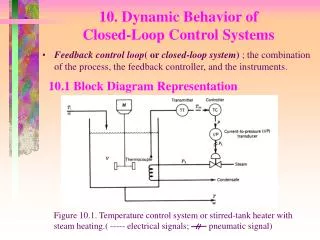
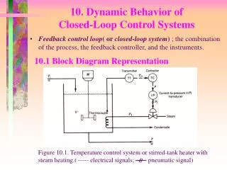
Figure 10.1. Temperature control system or stirred-tank heater with steam heating.( ----- electrical signals; pneumatic signal). 10. Dynamic Behavior of Closed-Loop Control Systems.

E N D
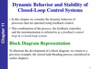
Figure 10.1. Temperature control system or stirred-tank heater with steam heating.( ----- electrical signals; pneumatic signal) 10. Dynamic Behavior of Closed-Loop Control Systems • Feedback control loop( or closed-loop system) ; the combination of the process, the feedback controller, and the instruments. 10.1 Block Diagram Representation
Process Where the subscripts , , and refer respectively to the wall of the heating coil, and to its steam and process sides. 10.1.1 Process Figure 10.2. Inputs and output of the process. • Dynamic model of a steam-heated, stirred tank:
Where is defined by • Assume that . • Assume that the dynamics of the heating coil are negligible since the dynamics are fast compared to the dynamics of the tank contents. Left side of (10.2) equal to zero! Substituting (10.4) into (10.1) gives
Apply Laplace transform after introducing deviation variables. where Figure 10.3. Block diagram of the process.
If negligible dynamics. • Steady-state gain depends on the input and output ranges of the thermocouple-transmitter combination. 10.1.2 Thermocouple and Transmitter • Assume that the dynamic behavior of the thermocouple and transmitter can be approximated by a first-order transfer function: Figure 10.4. Block diagram for the thermocouple and temperature transmitter.
where and are the Laplace transforms of the controller output and error signal . Note that and are electrical signals which have the units of [mA] while is dimensionless. 10.1.3 Controller • Assume that a proportional plus integral controller is used Figure 10.5. Block diagram for the controller.
Since transducers are usually designed to have linear characteristics and negligible(fast) dynamics Assume that the transducer transfer function merely consists of a steady-state gain : 10.1.5 Control Valve The flow through the valve is a non-linear function of the signal to the valve actuator. However, a first-order transfer function usually provides an adequate model for operation of an installed valve in the vicinity of a nominal steady-state. 10.1.4 Current-to-Pressure(I/P) Transducer Figure 10.6. Block diagram for the I/P transducer. Figure 10.7. Block diagram for the control valve.
Complete block diagram Figure 10.8. Block diagram for the entire control system.
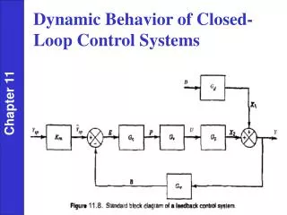
= Controlled variable = Manipulated variable = Load variable = Controller output = Error signal = Change in due to = Internal set point(used by controller) = Measured value of = Set point = Change in due to = Set point = Process transfer function = Transfer function for final control element = Steady-state gain for = Load transfer function = Transfer function for measuring element and transmitter 10.2 Closed-Loop Transfer Functions • The standard notations.
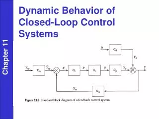
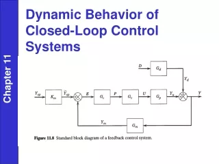
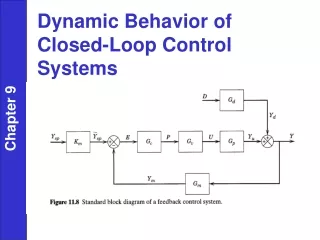
Figure 10.9. Standard block diagram of a feedback control system • In Figure 10.9. each variable is the Laplace Transform of a deviation variable. • Feedforward path: the signal path from to through blocks , and . • Feedback path: the signal path from to the comparator through .
For these two block diagrams to be equivalent, the relation between and must be preserved. Thus, and must be related by the expression. Figure 10.10. Alternative form of the standard block diagram of a feedback control system
By successive substitution, Figure 10.12. Equivalent block diagram. 10.2.1 Block Diagram Reduction • It is often convenient to combine several blocks into a single block. • Example Figure 10.11. Three blocks in series.
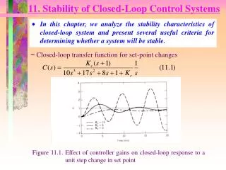
10.2.2 Set Point Changes( = Servo Problem) Figure 10.9. Standard block diagram of a feedback control system • Desired closed-loop transfer function,
A comparison of (10.23) and (10.25) indicate that both closed-loop transfer functions have the same denominator. The denominator is written as where is the open-loop transfer function, . 10.2.2 Load Changes( = Regulatory Problem) • Desired closed-loop transfer function,
10.3 Closed-loop Responses of Simple Control Systems In this section, we consider the dynamic behavior of several elementary control problems for load variable and set-point changes. • For the liquid-level control system Figure 10.10. Liquid-level Control System
q1: the load variable. q2: the manipulated variable. Assumption: 1. The liquid density r and the cross-sectional area of the tank A are constant. 2. The flow-head relation is linear, q3 = h/R. 3. The transmitter and control valves have negligible dynamics. 4. Pneumatic instruments are used. • Mass balance for the tank contents. • Transfer Function Where, KP= R, t = RA
Assuming that the dynamics of the level transmitter and control valve, the corresponding transfer functions can be written as Gm(s) = Km and Gv(s) = Kv . • Block diagram for level control system Figure 10.11. Block diagram for level control system
Proportional Control and Set-Point Change If a proportional controller is used, then Gc(s) = Kc . The closed-loop transfer function for set-point changes is given by where, KOLis the open-loop gain, KOL =Kc Kv Kp Km (KOL > 0 for stability → chapter 11) Thus since t1 < t , one consequence of feedback control is that it enables the controlled process to respond more quickly than the uncontrolled process. The reason for the introduction of feedback control
The closed-loop response to a unit step change of magnitude M in set point is given by Figure 10.12. Step response for proportional control (set-point change)
The offset ( steady-state error) is defined as Since KOL =Kc Kv Kp Km Kc : , KOL : , offset : if Kc , offset 0
Proportional Control and Load Changes The closed-loop transfer function for load changes is given by where, The closed-loop response to step change of magnitude M in load The same situation can be observed as set point change case
PI Control and Load Changes The closed-loop transfer function for load change is given by This transfer function can be rearranged as a second-order one. where, K3 = tI / KcKvKm
For a unit step change in load, because of the exponential term in (10.39). For set-point change, offset will be zero too! Addition of Integral action Elimination of offset for step changes of load and set-point
PI Control of an Integrating Process Figure 10.13. Liquid-level control system with pump in exit line This system differs from the previous example in two ways 1. The exit line contains a pump 2. The manipulated variable is the exit flow rate rather than an inlet flow rate.
The process and load transfer functions are given by The closed-loop transfer function for load changes where, K4 = -tI / KcKvKm KOL = KcKvKpKm , Kp = - 1/A
The effect of tI tI: : closed-loop responses: less oscillatory • The effect of Kc Kc: z4: closed-loop responses: less oscillatory • The effect of Kc for the stable process except the integrating process Kc: closed-loop responses: more oscillatory