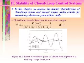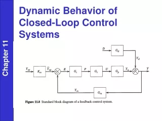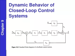
Specifications and closed-loop control
Specifications and closed-loop control. Specifications: Basic terminology. Resolution: value of smallest resolvable displacement (step) of the component; it differs from the resolution of the measurement

Specifications and closed-loop control
E N D
Presentation Transcript
Specifications:Basic terminology Resolution: value of smallest resolvable displacement (step) of the component; it differs from the resolution of the measurement Accuracy (error): difference between the (mean) actual motion and the ideal displacement of the device Repeatability (precision): range of deviations of the actual displacement for the same nominal (error free) displacement
Specifications:Basic terminology Resolution: largest of the smallest steps the device can make (smallest programmable step) during point-to-point motion Accuracy (error): maximum error between any 2 points in the work volume, i.e. difference between the mean value of the reached positions and the nominal position Repeatability (precision): error between a number of successive attempts to move to the same position
How to reach specifications • Precise actuation only? • Move until you think you have reached the target position (called „open-loop control“) • This works only sometimes. • For precision system even more seldom. Position, force, etc. System Actuation
A D Problems with open-loop control:example 1 The actuation is either not accurate (but you could calibrate) or not precise. Example: The resolution of your actuation is not sufficient 12 bits actuation, position with higher resolution needed
Problems with open-loop control:example 2 The system may be affected by external disturbances Example: The mass spring system at the right is affected by the weight Affected by weight of mass (causes unwanted displacement) Not affected
Problems with open-loop control:example 3 The system is slightly different from what imagined Example: The spring constant k of the mass spring system is different from what assumed. The same force causes a different displacement. Example: The spring constant k varies with the displacement. Increasing the force does not increase the displacement proportionally.
Problems with open-loop control:example 4 You may want to reach the end position faster (dynamics is not satisfactory) Example: When system shows slightly damped oscillations, like in flexure systems.
Problems with open-loop control:example 5 The system is unstable: the desired position can not be achieved Example: The magnetically levitated ball is attracted by the magnet if too close to magnet, falls down if too far from the magnet.
Closed-loop control • Use information from measurements! • Build error e between reference r (desired value) and measured value y • Use this error somehow to influence the actuation u Many problems can be solved with closed-loop control
D A A D Problems solved withclosed-loop control: example 1 The actuation is either not accurate or not precise. Example: It is possible to obtain a high resolution reference voltage using high resolution AD converters, even with low resolution DA converters. High resolution voltage! + Low passfilter controller -
Problems solved withclosed-loop control: example 2 The system may be affected by external disturbances Example: The extra displacement caused by the weight can be perfectly compensated in any position Affected by weight of mass No unwanted displacement Not affected
Problems solved withclosed-loop control: example 3 The system is slightly different from what imagined Example: The closed-loop control can take care of varying of uncertain spring constant values k
Problems solved withclosed-loop control: example 4 You may want to reach the end position faster (dynamics is not satisfactory) Example: Closed-loop control can effectively damp oscillations, even change bandwith.
Problems solved withclosed-loop control: example 5 The open-loop system is unstable Example: The magnetically levitated ball can be kept floating at a given position
Limitations inclosed-loop control systems However, not everything is possible Example: closed-loop control cannot cure deficiencies in the system repeatability or in the measurement accuracy Example: With given measurement noise, the achievable bandwidth is limited (trade-off) Example: Stability and performance are competing (trade-off)
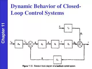
Plant with controller d r u y Controller Plant w r: reference signal u: command signal w: measured signal y: output signal d: disturbance
Control problem Given PlantG(s), find controllerC(s) such that closed-loop system with transfer function satisfies behavior specifications
Feedforward scheme Closed-loop system with transfer function
Advantages ofFeedforward scheme • Poles still determined by G(s) and C(s)Closed-loop bandwidth may be reduced, which improves noise rejection (see later) • F2(s)already generates the necessary actuation,C(s)is responsible only for deviations better response, less problems, better accuracy • F1(s) „conditions“ the reference by filtering it (same must be done byF2(s)) Sharp changes inR(s) don‘t cause abrupt changes in actuation
Advantages ofCompensation scheme • Closed-loop behavior still determined by Gyu(s) and C(s)Closed-loop bandwidth may be reduced, which improves noise rejection (see later) • H(s)already generates the necessary actuation,C(s)is responsible only for deviations better response to disturbance changes, less problems, better accuracy
Setup Objective: output yshould follow desired or commanded signal r while not using too much control effort u! disturbances Plant uncertainty Measurement noise Robust performance=command following+disturbance rejection,despite of plant variations
Major transfer functions • Loop gainL(s)=P(s).C(s) • Sensitivity functionS(s)=1/(1+L(s))=1/(1+P(s).C(s)) • Complementary sensitivity functionT(s)=L(s)/(1+L(s))=P(s).C(s)/(1+P(s).C(s))
S(s) reduces the influence of disturbances T(s) non–zero: measurementnoise affects the output (unlike open-loop) Nominal signal response (1) Output
S(s) small with respect to reference and disturbances T(s) small with respect to noise Nominal signal response (2) - + eP(s) Performance error
Nominal signal response (3) Command input(actuation) • V(s) increases asP(s)decreases in frequency (usual case), unlessT(s) also decreases or r(s),do(s)and(s)also decrease • As (s)increases in frequency,T(s) must decrease • bandwidth limitation!
Limitation 1 • high-frequency measurement noise (t) or disturbances di(t) or do(t) and • Limitations on the desired control magnitude v(t) • Limitation of bandwidth on theclosed-loop system
Sensitivity to plant variations Plant variations causes variations |S(jw)|<1 feedback decreases effect |S(jw)|>1 feedback increases effect
Robust stability T(s) Suppose we know(uncertainty is limited) Then stability requires (justification e.g. with Nyquist diagram, not presented here)
Specifications So, because of plant variations... • S(jw) should be small ( ) maxizimize benefits (disturbance rejection, command following, performance) • T(jw) should be small ( ) minimize costs (noise amplification, instability, control effort, ...)
Limitation 2 But So, specifications are tradeoffs! S(jw) and T(jw) can’t be both small at same w
Limitation 2 However Disturbance rejection and command following ar important at low frequencies S(jw) small at low frequencies Uncertainty and measurement noise important a high frequencies T(jw) small at high frequencies
Specifications on Loop gain (1) For low frequency
Specifications on Loop gain (2) For high frequency
Specifications on Loop gain (3) At crossover Undesirable Condition on phase
Bode Gain-Phase Relation If no pole and right half-plane zeros where Phase completely determined by (weighted) Integral of derivative of log amplitude In fact 20n db/decade decrease
Bode Gain-Phase Relation (2):crossover slope As angle at crossover must be between –p and p Bode rate decrease must be 20 db/decade at crossover 20dB/decade
50 50 50 50 ! High decrease rate 0 0 0 0 -50 -50 -50 -50 -100 -100 -100 -100 Magnitude (dB) Magnitude (dB) Magnitude (dB) Magnitude (dB) -150 -150 -150 -150 -200 -200 -200 -200 -250 -250 -250 -250 0 0 0 0 2 2 2 2 4 4 4 4 6 6 6 6 10 10 10 10 10 10 10 10 10 10 10 10 10 10 10 10 Bode Gain-Phase Relation (3)crossover slope
50 50 50 same high decrease ratespecs 100dB higher 0 0 0 -50 -50 -50 -100 -100 -100 Magnitude (dB) Magnitude (dB) Magnitude (dB) -150 -150 -150 -200 -200 -200 -250 -250 -250 0 0 0 2 2 2 4 4 4 6 6 6 10 10 10 10 10 10 10 10 10 10 10 10 Bode Gain-Phase Relation (4)crossover slope, narrower specs
Bode Sensitivity integral If relative degree at least 2 (2 more poles than zeroes) and no right-half plane poles (stable plant) Tradeoff between sensitivity properties in different frequency ranges
Bode Sensitivity integral for Green surfacec exactly compensates red one