Dynamic Behavior of Closed-Loop Control Systems
630 likes | 937 Vues
Explore the dynamic behavior and stability of processes using feedback control in closed-loop systems. Learn block diagram representations and transfer functions for various system elements for effective control. Understand how controllers, transducers, and valves contribute to system performance and stability.

Dynamic Behavior of Closed-Loop Control Systems
E N D
Presentation Transcript
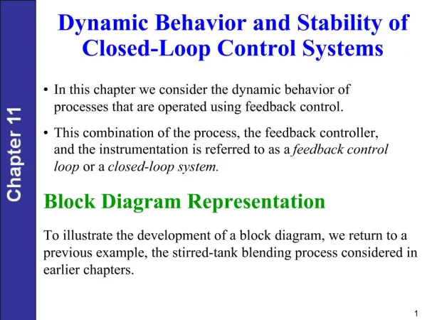
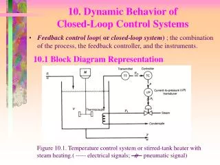
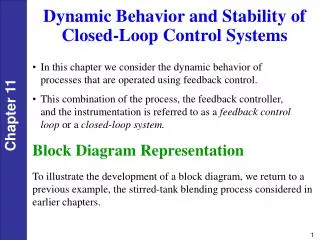
Dynamic Behavior and Stability of Closed-Loop Control Systems • In this chapter we consider the dynamic behavior of processes that are operated using feedback control. • This combination of the process, the feedback controller, and the instrumentation is referred to as a feedback control loop or a closed-loop system. Block Diagram Representation To illustrate the development of a block diagram, we return to a previous example, the stirred-tank blending process considered in earlier chapters.
Figure 11.1 Composition control system for a stirred-tank blending process.
Next, we develop a transfer function for each of the five elements in the feedback control loop. For the sake of simplicity, flow rate w1 is assumed to be constant, and the system is initially operating at the nominal steady rate. Process In section 4.3 the approximate dynamic model of a stirred-tank blending system was developed: where
Composition Sensor-Transmitter (Analyzer) We assume that the dynamic behavior of the composition sensor-transmitter can be approximated by a first-order transfer function: Controller Suppose that an electronic proportional plus integral controller is used. From Chapter 8, the controller transfer function is where and E(s) are the Laplace transforms of the controller output and the error signal e(t). Note that and e are electrical signals that have units of mA, while Kc is dimensionless. The error signal is expressed as
or after taking Laplace transforms, The symbol denotes the internal set-point composition expressed as an equivalent electrical current signal. This signal is used internally by the controller. is related to the actual composition set point by the composition sensor-transmitter gain Km: Thus
Figure 11.3 Block diagram for the composition sensor-transmitter (analyzer).
Current-to-Pressure (I/P) Transducer Because transducers are usually designed to have linear characteristics and negligible (fast) dynamics, we assume that the transducer transfer function merely consists of a steady-state gain KIP: Control Valve As discussed in Section 9.2, control valves are usually designed so that the flow rate through the valve is a nearly linear function of the signal to the valve actuator. Therefore, a first-order transfer function usually provides an adequate model for operation of an installed valve in the vicinity of a nominal steady state. Thus, we assume that the control valve can be modeled as
Figure 11.5 Block diagram for the I/P transducer. Figure 11.6 Block diagram for the control valve.
Figure 11.7 Block diagram for the entire blending process composition control system.
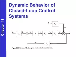
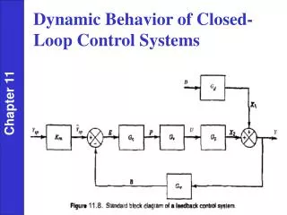
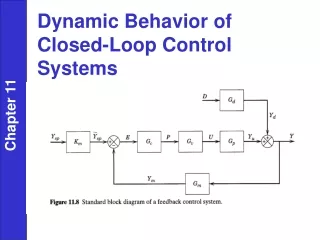
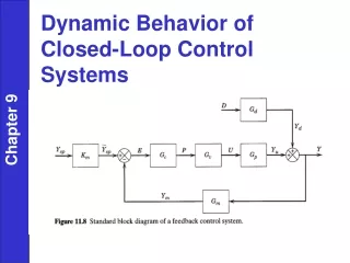
Closed-Loop Transfer Functions The block diagrams considered so far have been specifically developed for the stirred-tank blending system. The more general block diagram in Fig. 11.8 contains the standard notation:
Figure 11.8 Standard block diagram of a feedback control system.
Block Diagram Reduction In deriving closed-loop transfer functions, it is often convenient to combine several blocks into a single block. For example, consider the three blocks in series in Fig. 11.10. The block diagram indicates the following relations: By successive substitution, or where
Figure 11.10 Three blocks in series. Figure 11.11 Equivalent block diagram.
Set-Point Changes Next we derive the closed-loop transfer function for set-point changes. The closed-loop system behavior for set-point changes is also referred to as the servomechanism (servo) problem in the control literature. Combining gives
Figure 11.8 also indicates the following input/output relations for the individual blocks: Combining the above equations gives
Rearranging gives the desired closed-loop transfer function, Disturbance Changes Now consider the case of disturbance changes, which is also referred to as the regulator problem since the process is to be regulated at a constant set point. From Fig. 11.8, Substituting (11-18) through (11-22) gives
Because Ysp = 0 we can arrange (11-28) to give the closed-loop transfer function for disturbance changes: A comparison of Eqs. 11-26 and 11-29 indicates that both closed-loop transfer functions have the same denominator, 1 + GcGvGpGm. The denominator is often written as 1 + GOL where GOL is the open-loop transfer function, At different points in the above derivations, we assumed that D = 0 or Ysp = 0, that is, that one of the two inputs was constant. But suppose that D≠ 0 and Ysp ≠ 0, as would be the case if a disturbance occurs during a set-point change. To analyze this situation, we rearrange Eq. 11-28 and substitute the definition of GOL to obtain
Thus, the response to simultaneous disturbance variable and set-point changes is merely the sum of the individual responses, as can be seen by comparing Eqs. 11-26, 11-29, and 11-30. This result is a consequence of the Superposition Principle for linear systems.
General Expression for Feedback Control Systems Closed-loop transfer functions for more complicated block diagrams can be written in the general form: where:
Example 11.1 Find the closed-loop transfer function Y/Yspfor the complex control system in Figure 11.12. Notice that this block diagram has two feedback loops and two disturbance variables. This configuration arises when the cascade control scheme of Chapter 16 is employed. Figure 11.12 Complex control system.
Solution Using the general rule in (11-31), we first reduce the inner loop to a single block as shown in Fig. 11.13. To solve the servo problem, set D1 = D2 = 0. Because Fig. 11.13 contains a single feedback loop, use (11-31) to obtain Fig. 11.14a. The final block diagram is shown in Fig. 11.14b with Y/Ysp = Km1G5. Substitution for G4 and G5 gives the desired closed-loop transfer function: Closed-Loop Responses of Simple Control Systems In this section we consider the dynamic behavior of several elementary control problems for disturbance variable and set-point changes.
The transient responses can be determined in a straightforward manner if the closed-loop transfer functions are available. Consider the liquid-level control system shown in Fig. 11.15. The liquid level is measured and the level transmitter (LT) output is sent to a feedback controller (LC) that controls liquid level by adjusting volumetric flow rate q2. A second inlet flow rate q1 is the disturbance variable. Assume: • The liquid density r and the cross-sectional area of the tank A are constant. • The flow-head relation is linear, q3 = h/R. • The level transmitter, I/P transducer, and control valve have negligible dynamics. • An electronic controller with input and output in % is used (full scale = 100%).
Derivation of the process and disturbance transfer functions directly follows Example 4.4. Consider the unsteady-state mass balance for the tank contents: Substituting the flow-head relation, q3 = h/R, and introducing deviation variables gives Thus, we obtain the transfer functions
where Kp = R and = RA. Note that Gp(s) and Gd(s) are identical because q1 and q2 are both inlet flow rates and thus have the same effect on h. Proportional Control and Set-Point Changes If a proportional controller is used, then Gc(s) = Kc. From Fig. 11.6 and the material in the previous section, it follows that the closed-loop transfer function for set-point changes is given by
This relation can be rearranged in the standard form for a first-order transfer function, where: and the open-loop gainKOL is given by
From Eq. 11-37 it follows that the closed-loop response to a unit step change of magnitude M in set point is given by This response is shown in Fig. 11.17. Note that a steady-state error or offset exists because the new steady-state value is K1M rather than the desired value of M. The offset is defined as For a step change of magnitude M in set point, . From (11-41), it is clear that . Substituting these values and (11-38) into (11-42) gives
Figure 11.17 Step response for proportional control (set-point change).
Proportional Control and Disturbance Changes From Fig. 11.16 and Eq. 11-29 the closed-loop transfer function for disturbance changes with proportional control is Rearranging gives where is defined in (11-39) and K2 is given by
A comparison of (11-54) and (11-37) indicates that both closed-loop transfer functions are first-order and have the same time constant. • However, the steady-state gains, K1 and K2, are different. • From Eq. 11-54 it follows that the closed-loop response to a step change in disturbance of magnitude M is given by The offset can be determined from Eq. 11-56. Now since we are considering disturbance changes and for a step change of magnitude M. Thus,
PI Control and Disturbance Changes For PI control, . The closed-loop transfer function for disturbance changes can then be derived from Fig. 11.16: Clearing terms in the denominator gives Further rearrangement allows the denominator to be placed in the standard form for a second-order transfer function:
where For a unit step change in disturbance, , and (11-59) becomes For , the response is a damped oscillation that can be described by
PI Control of an Integrating Process Consider the liquid-level control system shown in Fig. 11.22. This system differs from the previous example in two ways: • the exit line contains a pump and • the manipulated variable is the exit flow rate rather than an inlet flow rate. In Section 5.3 we saw that a tank with a pump in the exit stream can act as an integrator with respect to flow rate changes because
Figure 11.22 Liquid-level control system with pump in exit line.
If the level transmitter and control valve in Eq. 11.22 have negligible dynamics, the Gm(s) = Km and Gv(s) = Kv. For PI control, . Substituting these expressions into the closed-loop transfer function for disturbance changes and rearranging gives where And KOL = KcKvKpKm with Kp = - 1/A.
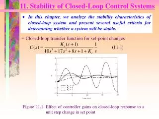
Stability of Closed-Loop Control Systems Example 11.4 Consider the feedback control system shown in Fig. 11.8 with the following transfer functions: Show that the closed-loop system produces unstable responses if controller gain Kc is too large.
Figure 11.23. Effect of controller gains on closed-loop response to a unit step change in set point (example 11.1).
Stability • Most industrial processes are stable without feedback control. Thus, they are said to be open-loop stable or self-regulating. • An open-loop stable process will return to the original steady state after a transient disturbance (one that is not sustained) occurs. • By contrast there are a few processes, such as exothermic chemical reactors, that can be open-loop unstable. Definition of Stability.An unconstrained linear system is said to be stable if the output response is bounded for all bounded inputs. Otherwise it is said to be unstable.
Characteristic Equation As a starting point for the stability analysis, consider the block diagram in Fig. 11.8. Using block diagram algebra that was developed earlier in this chapter, we obtain where GOL is the open-loop transfer function, GOL = GcGvGpGm. For the moment consider set-point changes only, in which case Eq. 11-80 reduces to the closed-loop transfer function,
Comparing Eqs. 11-81 and 11-82 indicates that the poles are also the roots of the following equation, which is referred to as the characteristic equation of the closed-loop system: General Stability Criterion.The feedback control system in Fig. 11.8 is stable if and only if all roots of the characteristic equation are negative or have negative real parts. Otherwise, the system is unstable. Example 11.8 Consider a process, Gp = 0.2/-s + 1), and thus is open-loop unstable. If Gv = Gm = 1, determine whether a proportional controller can stabilize the closed-loop system.
Figure 11.25 Stability regions in the complex plane for roots of the charact-eristic equation.
Figure 11.26 Contributions of characteristic equation roots to closed-loop response.
Solution The characteristic equation for this system is Which has the single root, s = -1 + 0.2Kc. Thus, the stability requirement is that Kc < 5. This example illustrates the important fact that feedback control can be used to stabilize a process that is not stable without control. Routh Stability Criterion The Routh stability criterion is based on a characteristic equation that has the form