Internet structure: network of networks
1.22k likes | 1.88k Vues
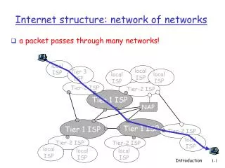
a packet passes through many networks!. Tier 3 ISP. local ISP. local ISP. local ISP. local ISP. local ISP. local ISP. local ISP. local ISP. NAP. Tier-2 ISP. Tier-2 ISP. Tier-2 ISP. Tier-2 ISP. Tier-2 ISP. Internet structure: network of networks. Tier 1 ISP. Tier 1 ISP.

Internet structure: network of networks
E N D
Presentation Transcript
a packet passes through many networks! Tier 3 ISP local ISP local ISP local ISP local ISP local ISP local ISP local ISP local ISP NAP Tier-2 ISP Tier-2 ISP Tier-2 ISP Tier-2 ISP Tier-2 ISP Internet structure: network of networks Tier 1 ISP Tier 1 ISP Tier 1 ISP Introduction
application: supporting network applications FTP, SMTP, HTTP transport: process-process data transfer TCP, UDP network: routing of datagrams from source to destination IP, routing protocols link: data transfer between neighboring network elements PPP, Ethernet physical: bits “on the wire” application transport network link physical Internet protocol stack Introduction
network link physical link physical M M M Ht M Hn Hn Hn Hn Ht Ht Ht Ht M M M M Ht Ht Hn Hl Hl Hl Hn Hn Hn Ht Ht Ht M M M source Encapsulation message application transport network link physical segment datagram frame switch destination application transport network link physical router Introduction
Chapter 2: applications Introduction
Architectures • Client-server • Peer-to-peer • Hybrid Introduction
HTTP: hypertext transfer protocol Web’s application layer protocol client/server model client: browser that requests, receives, “displays” Web objects server: Web server sends objects in response to requests HTTP 1.0: RFC 1945 HTTP 1.1: RFC 2068 HTTP overview Linux running Firefox HTTP request HTTP response HTTP request PC running Explorer HTTP response HTTP request Server running Apache Web server HTTP response Mac running Navigator Introduction
HTTP Review • TCP • “Stateless” • Non-persistent 44 messages, 22 RTT • Persistent 24 messages • Non-pipelined 12 RTT • Pipelined 3 RTT • HTTP Commands (GET, POST, HEAD, etc) • HTTP Fields (User-agent, Connection, etc) • Telnet as a command-line TCP connection Introduction
Cookie file Cookie file Cookie file ebay: 8734 amazon: 1678 ebay: 8734 amazon: 1678 ebay: 8734 cookie- specific action access usual http request msg cookie: 1678 usual http request msg cookie: 1678 access one week later: usual http response msg usual http response msg cookie- spectific action Cookies: keeping “state” (cont.) client server usual http request msg server creates ID 1678 for user entry in backend database usual http response + Set-cookie: 1678 Introduction
Install cache suppose hit rate is .4 Consequence 40% requests will be satisfied almost immediately 60% requests satisfied by origin server utilization of access link reduced to 60%, resulting in negligible delays (say 10 msec) total avg delay = Internet delay + access delay + LAN delay = .6*(2.01) secs + .4*milliseconds < 1.4 secs Optimization example (cont) origin servers public Internet 1.5 Mbps access link institutional network 10 Mbps LAN institutional cache Introduction
1) Alice uses UA to compose message and “to” bob@someschool.edu 2) Alice’s UA sends message to her mail server; message placed in message queue 3) Client side of SMTP opens TCP connection with Bob’s mail server 4) SMTP client sends Alice’s message over the TCP connection 5) Bob’s mail server places the message in Bob’s mailbox 6) Bob invokes his user agent to read message user agent user agent mail server mail server Scenario: Alice sends message to Bob 1 2 6 3 4 5 Introduction
Root DNS Servers org DNS servers edu DNS servers com DNS servers poly.edu DNS servers umass.edu DNS servers pbs.org DNS servers yahoo.com DNS servers amazon.com DNS servers Distributed, Hierarchical Database Client wants IP for www.amazon.com; 1st approx: • Client queries a root server to find com DNS server • Client queries com DNS server to get amazon.com DNS server • Client queries amazon.com DNS server to get IP address for www.amazon.com Introduction
root DNS server 2 3 6 7 TLD DNS server 4 local DNS server Cs.virginia.edu local DNS server Cs.virginia.edu 5 1 8 authoritative DNS server dns.cs.umass.edu requesting host Cs.virginia.edu gaia.cs.umass.edu Iterative Queries vs Recursive Queries root DNS server 2 3 TLD DNS server 4 5 6 7 1 8 authoritative DNS server dns.cs.umass.edu requesting host Cs.virginia.edu gaia.cs.umass.edu Introduction
Bob centralized directory server 1 peers 1 3 1 2 1 Alice P2P: centralized directory original “Napster” design 1) when peer connects, it informs central server: • IP address • content 2) Alice queries for “Hey Jude” 3) Alice requests file from Bob Introduction
Query QueryHit Query Query QueryHit Query QueryHit Query Gnutella: protocol File transfer: HTTP • Query messagesent over existing TCPconnections • peers forwardQuery message • QueryHit sent over reversepath Scalability: limited scopeflooding Introduction
Exploiting heterogeneity: KaZaA • Each peer is either a group leader or assigned to a group leader. • TCP connection between peer and its group leader. • TCP connections between some pairs of group leaders. • Group leader tracks the content in all its children. Introduction
Chapter 3: transport Introduction
Transport Layer Review • Connection-oriented (TCP) • Acknowledgements (can have retries) • Flow control • Congestion control • Better for most protocols • Connectionless (UDP) • No acknowledgements • Send as fast as needed • Some packets will get lost • Better for video, telephony, etc • Human speech? Introduction
P2 Connectionless demux (cont) DatagramSocket serverSocket = new DatagramSocket(6428); P1 P1 P3 SP: 6428 SP: 6428 DP: 9157 DP: 5775 SP: 9157 SP: 5775 client IP: A DP: 6428 DP: 6428 Client IP:B server IP: C SP provides “return address” Introduction
SP: 9157 SP: 5775 P1 P1 P2 P3 client IP: A DP: 80 DP: 80 Connection-oriented demux: Threaded Web Server P4 S-IP: B D-IP:C SP: 9157 DP: 80 Client IP:B server IP: C S-IP: A S-IP: B D-IP:C D-IP:C Introduction
Notice: • TCP sockets: • Server port required to create listening socket • Server address and port needed by client for connection setup • Nodes can talk freely after that • UDP sockets • Server port required to create listening socket • Every message requires dest address/port • All reads provide source address/port Introduction
Internet Checksum Example • Note • When adding numbers, a carryout from the most significant bit needs to be added to the result • Example: add two 16-bit integers 1 1 1 1 0 0 1 1 0 0 1 1 0 0 1 1 0 1 1 1 0 1 0 1 0 1 0 1 0 1 0 1 0 1 1 1 0 1 1 1 0 1 1 1 0 1 1 1 0 1 1 1 1 0 1 1 1 0 1 1 1 0 1 1 1 1 0 0 1 0 1 0 0 0 1 0 0 0 1 0 0 0 0 1 1 wraparound sum checksum Introduction
Reliable Transport • Mechanisms for Reliable Transport • Packet Corruption Acks/Nacks • Ack corruption Sequence #s • Loss Timeouts • Pipelining • Go-Back-N: cumulative acks, no rxr buffering • Selective Repeat: individual acks, rxr buffering • Must be careful that rxrWindow <= max seq no / 2 Introduction
Pipelining: increased utilization sender receiver first packet bit transmitted, t = 0 last bit transmitted, t = L / R first packet bit arrives RTT last packet bit arrives, send ACK last bit of 2nd packet arrives, send ACK last bit of 3rd packet arrives, send ACK ACK arrives, send next packet, t = RTT + L / R Increase utilization by a factor of 3! Introduction
Sender: ACK(n): ACKs all pkts up to, including seq # n - “cumulative ACK” may receive duplicate ACKs (see receiver) timer for each in-flight pkt timeout(n): retransmit pkt n and all higher seq # pkts in window Go-Back-N • k-bit seq # in pkt header • “window” of up to N, consecutive unack’ed pkts allowed Introduction
Selective repeat: sender, receiver windows Introduction
TCP ACK generation[RFC 1122, RFC 2581] TCP Receiver action Delayed ACK. Wait up to 500ms for next segment. If no next segment, send ACK Immediately send single cumulative ACK, ACKing both in-order segments Buffer packet. Immediately send duplicate ACK, indicating seq. # of next expected byte Immediate send ACK, provided that segment starts at lower end of gap Event at Receiver Arrival of in-order segment with expected seq #. All data up to expected seq # already ACKed Arrival of in-order segment with expected seq #. One other segment has ACK pending Arrival of out-of-order segment higher-than-expect seq. # . Gap detected Arrival of segment that partially or completely fills gap Introduction
(Suppose TCP receiver discards out-of-order segments) spare room in buffer = RcvWindow = RcvBuffer-[LastByteRcvd - LastByteRead] Rcvr advertises spare room by including value of RcvWindow in segments Sender limits unACKed data to RcvWindow guarantees receive buffer doesn’t overflow TCP Flow control: how it works Introduction
Host A Host B Causes/costs of congestion: scenario 3 lout Another “cost” of congestion: • when packet dropped, any “upstream transmission capacity used for that packet was wasted! Introduction
Conservative on Timeout • After 3 dup ACKs: • CongWin is cut in half • window then grows linearly • But after timeout event: • CongWin instead set to 1 MSS; • window then grows exponentially • to a threshold, then grows linearly Philosophy: • 3 dup ACKs indicates network capable of delivering some segments • timeout indicates a “more alarming” congestion scenario Introduction
Summary: TCP Congestion Control • When CongWin is below Threshold, sender in slow-start phase, window grows exponentially. • When CongWin is above Threshold, sender is in congestion-avoidance phase, window grows linearly. • When a triple duplicate ACK occurs, Threshold set to CongWin/2 and CongWin set to Threshold. • When timeout occurs, Threshold set to CongWin/2 and CongWin is set to 1 MSS. Introduction
TCP sender congestion control Introduction
Two competing sessions: Additive increase gives slope of 1, as throughout increases multiplicative decrease decreases throughput proportionally Why is TCP fair? equal bandwidth share R loss: decrease window by factor of 2 congestion avoidance: additive increase Connection 2 throughput loss: decrease window by factor of 2 congestion avoidance: additive increase Connection 1 throughput R Introduction
Second case: WS/R < RTT + S/R: wait for ACK after sending window’s worth of data sent K is number of windows that cover the object For fixed W K=O/(WS) Fixed congestion window (2) delay = 2RTT + O/R + (K-1)[S/R + RTT - WS/R] Introduction
TCP Delay Modeling (3) Introduction
Chapter 4: Network Layer Introduction
used to setup, maintain teardown VC used in ATM, frame-relay, X.25 not used in today’s Internet application transport network data link physical application transport network data link physical Virtual circuits: signaling protocols 6. Receive data 5. Data flow begins 4. Call connected 3. Accept call 1. Initiate call 2. incoming call Introduction
no call setup or network-level concept of “connection” packets forwarded using destination host address packets between same source-dest pair may take different paths application transport network data link physical application transport network data link physical Datagram networks 1. Send data 2. Receive data Introduction
Comparison • Circuit Switching • Dedicated resources guarantees • wasted resource • setup delays • Packet Switching • On-demand resources no guarantees • congestion • store and forward delays Introduction
1. nodal processing: check bit errors determine output link Four sources of packet delay • 2. queueing • time waiting at output link for transmission • depends on congestion level of router A B nodal processing queueing Introduction
3. Transmission delay: R=link bandwidth (bps) L=packet length (bits) time to send bits into link = L/R 4. Propagation delay: d = length of physical link s = propagation speed in medium (~2x10⁸ m/sec) propagation delay = d/s Delay in packet-switched networks Note: s and R are very different quantities! transmission A propagation B nodal processing queueing Introduction
packet arrival rate to link exceeds output link capacity Queue grows When no more space in queue, packets are lost lost packet may be retransmitted by previous node, by source end system, or not retransmitted at all packets queueing (delay) free (available) buffers: arriving packets dropped (loss) if no free buffers How does loss occur? A B Introduction
Input Port Queuing • Fabric slower than input ports combined -> queueing may occur at input queues • Head-of-the-Line (HOL) blocking: queued datagram at front of queue prevents others in queue from moving forward • queueing delay and loss due to input buffer overflow! Introduction
Output port queueing • buffering when arrival rate via switch exceeds output line speed • queueing (delay) and loss due to output port buffer overflow! Introduction
host part subnet part 11001000 0001011100010000 00000000 200.23.16.0/23 IP addressing: CIDR CIDR:Classless InterDomain Routing • subnet portion of address of arbitrary length • address format: a.b.c.d/x, where x is # bits in subnet portion of address Introduction
200.23.16.0/23 200.23.18.0/23 200.23.30.0/23 200.23.20.0/23 . . . . . . Hierarchical addressing: route aggregation Hierarchical addressing allows efficient advertisement of routing information: Organization 0 Organization 1 “Send me anything with addresses beginning 200.23.16.0/20” Organization 2 Fly-By-Night-ISP Internet Organization 7 “Send me anything with addresses beginning 199.31.0.0/16” ISPs-R-Us Introduction
2 4 1 3 S: 138.76.29.7, 5001 D: 128.119.40.186, 80 S: 10.0.0.1, 3345 D: 128.119.40.186, 80 1: host 10.0.0.1 sends datagram to 128.119.40.186, 80 2: NAT router changes datagram source addr from 10.0.0.1, 3345 to 138.76.29.7, 5001, updates table S: 128.119.40.186, 80 D: 10.0.0.1, 3345 S: 128.119.40.186, 80 D: 138.76.29.7, 5001 NAT: Network Address Translation NAT translation table WAN side addr LAN side addr 138.76.29.7, 5001 10.0.0.1, 3345 …… …… 10.0.0.1 10.0.0.4 10.0.0.2 138.76.29.7 10.0.0.3 4: NAT router changes datagram dest addr from 138.76.29.7, 5001 to 10.0.0.1, 3345 3: Reply arrives dest. address: 138.76.29.7, 5001 Introduction
Flow: X Src: A Dest: F data Flow: X Src: A Dest: F data Flow: X Src: A Dest: F data Flow: X Src: A Dest: F data A B E F F A B E C D Src:B Dest: E Src:B Dest: E Tunneling tunnel Logical view: IPv6 IPv6 IPv6 IPv6 Physical view: IPv6 IPv6 IPv6 IPv6 IPv4 IPv4 A-to-B: IPv6 E-to-F: IPv6 B-to-C: IPv6 inside IPv4 B-to-C: IPv6 inside IPv4 Introduction
routing algorithm local forwarding table header value output link 0100 0101 0111 1001 3 2 2 1 value in arriving packet’s header 1 0111 2 3 Interplay between routing and forwarding Introduction
5 3 5 2 2 1 3 1 2 1 x z w u y v Dijkstra’s algorithm D(v),p(v) 2,u 2,u 2,u D(x),p(x) 1,u D(w),p(w) 5,u 4,x 3,y 3,y D(y),p(y) ∞ 2,x Step 0 1 2 3 4 5 N' u ux uxy uxyv uxyvw uxyvwz D(z),p(z) ∞ ∞ 4,y 4,y 4,y How to convert this into a routing table? Introduction
Oscillations possible: e.g., link cost = amount of carried traffic A A A A D D D D B B B B C C C C Dijkstra’s algorithm, discussion 1 1+e 2+e 0 2+e 0 2+e 0 0 0 1 1+e 0 0 1 1+e e 0 0 0 e 1 1+e 0 1 1 e … recompute … recompute routing … recompute initially Human Analogy? Introduction