Download
1 / 14
160 likes | 620 Vues
Cost of Capital. Cost of Equity. Dividend Valuation Model: Assume Re 1 share quoted at Rs. 2.50, dividend just paid Rs. 0.20. Cost of Equity. Dividend Growth Model: Assume Re 1 share quoted at Rs. 2.50, dividend just paid Rs. 0.20. Expected annual growth rate for the dividend is 5 per cent.

E N D
Cost of Equity • Dividend Valuation Model: • Assume Re 1 share quoted at Rs. 2.50, dividend just paid Rs. 0.20
Cost of Equity • Dividend Growth Model: • Assume Re 1 share quoted at Rs. 2.50, dividend just paid Rs. 0.20. Expected annual growth rate for the dividend is 5 per cent.
Cost of Equity: Estimating The Growth Rate • Historical dividend: • Year 2005: Rs. 15,000; Year 2006: Rs. 15,500; Year 2007: Rs. 17,200; Year 2008: Rs. 18,100; Year 2009: Rs. 19,000 • Historical average annual growth is calculated using the compound interest formula.
Estimating Growth: Gordon’s Growth Model • Assumptions: • The entity must be all equity financed; • Retained profit is the only source of additional investment; • A constant proportion of each year’s earnings is retained for reinvestment; and • Projects financed from retained earnings earn a constant rate of return
Estimating Growth: Gordon’s Growth Mod • An entity retains 60 per cent of its earnings for identified capital investment projects that are estimated to have an average post-tax return of 12 per cent.
Cost of Equity: • Capital Asset Pricing Model
Cost of Irredeemable Debt • Kd net = Cost of debt (after tax) • i= annual interest • t= rate of corporation tax (assumed immediately recoverable) • P0 = market value of debt (ex-interest, immediately after payment) • Assume 7 per cent bond quoted at cumulative interest market price of Rs. 90 and corporation tax is 30 per cent
Cost of Redeemable Debt • The cost of redeemable debt is calculated using an internal rate of return (IRR) approach. • The calculation takes the IRR of • the annual net of tax interest payments from year 1 to year n, plus • the redemption payment in year n, minus • the original market value of the debt in year zero
Cost of Convertible Debt • In the case of convertible bonds, the redemption payment would become the market value at year n of the ordinary shares into which the debt is to be converted . • We may calculate MV in n year’s time using the model:
Cost of Preference Shares • Kpref = cost of preference shares • d = annual dividend • P0 = current ex-dividend market price
Modigliani and Millers’ Theories of Gearing • Proposition I • The market value of any entity is independent of its capital structure and is given by capitalizing its expected return at the rate appropriate to its class. • Vg = Vug • Proposition II • The expected yield of a share is equal to the appropriate capitalization rate for a pure equity stream in the class, plus a premium related to financial risk equal to the debt-to equity ratio times the spread between the capitalisation rate and the interest rate on debt. • Keg = keu + (D/E)×( keu – kd)
Modigliani and Millers’ Theories of Gearing (Contd.) • Proposition III • The cut-off point for investment in the entity will in all cases be the average cost of capital and will be completely unaffected by the type of security used to finance the investment. • WACCg = WACCug
Modigliani and Millers’ Theories of Gearing :With Tax • Proposition I • Vg = Vug + TB • TB = Present Value of Tax Shield • Proposition II • keg = keu + [(1 – t)× (D/E)×( keu – kd)] • Proposition III • WACCg = WACCug × [1 – TB/(D+E)] • Or • WACCg = [keg× (E/(D+E)] + [kd× (1 –t)× (D(D+E)]