Download
1 / 115
1.18k likes | 1.38k Vues
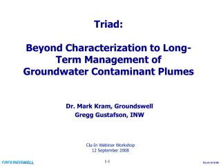
Triad: Beyond Characterization to Long-Term Management of Groundwater Contaminant Plumes. Dr. Mark Kram, Groundswell Gregg Gustafson, INW. Clu-In Webinar Workshop 12 September 2008. 1-1. Present a comprehensive approach to optimized characterization/remediation design/LTM

E N D
Triad:Beyond Characterization to Long-Term Management ofGroundwater Contaminant Plumes Dr. Mark Kram, Groundswell Gregg Gustafson, INW Clu-In Webinar Workshop 12 September 2008 1-1
Present a comprehensive approach to optimized characterization/remediation design/LTM Take Triad to next level Use Triad based approaches to develop CSM Use CSM to develop remediation and monitoring strategy Integrate Triad/CSM/LTM components into streamlined process Work towards single mobilization solutions TECHNICAL OBJECTIVES 1-2
Innovative Direct Push Characterization Techniques Chemical Distributions (MIP, LIF, FFD, UVOST, GeoVIS, ConeSipper, WaterlooAPS Profiler) Hydraulic Parameter Distributions (HRP, HPT) 3D Flux Model Generation LTM Network Design Spatial Considerations (2D/3D) Well Design (ASTM vs. WDS) Sensor Technologies Desktop Monitoring Analytes (Today and in Near Future) Components of a Wireless Telemetry System New LTM Approaches Automation Rapid Reporting/Assessment/Lines of Evidence For additional information: http://clu-in.org/char/technologies/dpanalytical.cfm OUTLINE 1-3
Overview of an L&D Plume:Massachusetts Military Reservation (MMR) Site Adapted from CH2MHill, AFCEE 1-4
Numerous large & dilute TCE plumes Some plumes 2 miles long Using Pump & Treat for 10 years Over $400 million has been spent to date on investigation and cleanup The estimated total long term cost: $850 million Current status: 12 plumes require LTM (at least) Massachusetts Military Reservation Adapted from CH2MHill, AFCEE 1-5
Seepage velocity (): Ki where: K = hydraulic conductivity = ------ (length/time) i = hydraulic gradient = effective porosity Contaminant flux (F): F = [X] where: = seepage velocity (length/time; m/s) (mass/length2-time; mg/m2-s) [X] = concentration of solute (mass/volume; mg/m3) SEEPAGE VELOCITY AND FLUX 1-6
CONCENTRATION VS. FLUX Length F, 1-7
CONCENTRATION VS. FLUX Length F, High Concentration High Risk!! Concentration and Hydraulic Component 1-8
STREAMLINED APPROACH • Plume Delineation • MIP, LIF, ConeSipper, Field Lab, etc. • 2D/3D Concentration Representations • CPT Data for Well Design • Hydro Assessment • High-Res Piezocone (2D/3D Flow Field, K, head, eff. Por.) • Conventional Approaches (e.g., Wells, Aq. Tests, etc.) • LTM Network Design • WDS based on CPT Data • G.S.D. via ASTM D5092 • Field Installations (Clustered Short Screened Wells) • Surveys (Lat/Long/Elevation) • GMS Interpolations (, F), Initial Models 1-9
GW Plume Characterization Strategy D B C Wiedemeier et al., 1996 3D – Depth Specific Info; Wells or Continuous Profile 1-10
GW Plume Characterization Strategy D B C Wiedemeier et al., 1996 3D – Depth Specific Info; Wells or Continuous Profile 1-11
CONE PENETROMETER Self-Contained Field Lab: Soil Type, Chemistry, Samples, Wells, Hydrogeology, Tracer Injection, Amendments, etc. 1-12
FLUORESCENCE PROBES Fiber optic-based chemical sensor probe equipped with sapphire window; Light source induces fluorescence; Signal returns to surface for depth discrete analysis; Can be coupled with additional sensors (soil type, video, etc.). 1-13
LIF DataRemediation Performance(BeforeandAfterSteam Enhanced Extraction) 1-15
FLUORESCENCE PROBES Pro: NAPL evidence based on sensitive UV fluorescence of fuel constituents or co-mingled materials (multi-ring fuel compounds, etc.); Can rapidly measure in real time; Depth discrete signals; Can be coupled with lithologic sensors for correlation, well design; Good screening method with high resolution; Can use several off-the-shelf energy sources (UVOST, FFD, LIF); Cal EPA Certification and ASTM Standard. Con: Limited by lithology; False negatives and positives possible due to wavelength dependency; Not analyte-specific; Semi-quantitative so requires confirmation samples. 1-16
GeoVIS 1-17
Box is 2.5mm x 2mm 1-18
GeoVIS Pro: Unique perspective regarding subsurface reality; Only true NAPL confirmation tool; Can generate continuous graphic profile; Can provide some hydro info (porosity, g.s.d., NAPL saturation). Con: Rate of data collection limited by ability to visibly process information; Transparent NAPL droplets can be present and not detectable in current configuration; Limited by lithology; Porosity estimates poor in silty sands; Semi-quantitative assessment; Pressure or heat front may force droplets away from window. 1-19
Screening tool with semi-quantitative capabilities. Membrane is semi-permeable and is comprised of a thin film polymer impregnated into a stainless steel screen for support. The membrane is placed in a heated block attached to the probe and heated to approximately 100-120 degrees C. Analyses of vapors at surface via GC and various detectors. Membrane Interface Probe 1-20
MIP Pro: Excellent chemical screening tool; Can generate continuous profile or focus on specific depth; Analyte specific; Many types of analytes (VOCs, semi-VOCs); Can be coupled with lithologic sensors for correlation. Con: When operating with a non-continuous configuration, user needs to determine appropriate target sample depths while “on the fly”; Constant operational conditions not always possible; Bulk fluids can not travel across membrane; Semi-quantitative; Clogging and carry-over can occur (some work-arounds); Limited by lithology; Heat front or pressure front may inhibit membrane contact with contaminant. 1-22
CONESIPPER • Soil-gas and water sampler; • Pneumatic valving; • 200 foot depth capacity; • Inert gas used to move samples to surface; • Up to 80ml samples; • Downhole decontamination; • Great for focused MIP confirmation. 1-23
CONESIPPER Pro: Depth discrete samples Vapor and liquid samples Can be coupled with rapid analyses (min. holding time concern) Excellent confirmation for MIP, UV Fluorescence, etc. Con: Decontamination concerns Single depth sample per push (not continuous) Not typically coupled with sensors (exceptions) Clogging can occur Limited by lithology (fines can be difficult) Pressure or heat front may cause displacement 1-24
WATERLOOAPS ADVANCED PROFILING SYSTEM • Collect samples • Couple with field analyses (GC, etc.) • Measure head • Measure index of K • Measure physicochem properties (pH, conductance, D.O., redox, T) via in-line flow-through cell • Can grout through tip 1-25
WATERLOOAPS ADVANCED PROFILING SYSTEM Pro: Depth discrete samples Vapor and liquid samples Can be coupled with rapid analyses (min. holding time concern) Hydro info (head, relative K) Excellent confirmation and CSM tool Con: Limited by lithology K values not quantified, so limited modeling capabilities Pressure or heat front may cause displacement 1-27
Direct-Push (DP) Sensor Probe that Converts Pore Pressure to Water Level or Hydraulic Head Head Values to ± 0.08ft (to >60’ below w.t.) Can Measure Vertical Gradients Simultaneously Collect Soil Type and K K from Pressure Dissipation, Soil Type Minimal Worker Exposure to Contaminants System Installed on NAVFAC SCAPS Licensed to AMS High-Resolution Piezocone Custom Transducer 1-28
PIEZOCONE OUTPUT Final Pressures Dissipation Tests 1-29
HRP TESTS(6/13/06) Head Values for Piezocone W2 W3 W1 Displays shallow gradient 1-30
Site Characterization with High Resolution Piezocone 11/22/04 Field Demo 6/13/06 Well Development & Hydraulic Test 8/24/05 Installation ¾” Wells 7/28/05 1st Wells 12/9/04 FIELD EFFORTS 1-31
HEAD DETERMINATION(3-D Interpolations) Piezo Wells • Shallow gradient (5.49-5.41’; 5.45-5.38’ range in clusters over 25’) • In practice, resolution exceptional (larger push spacing) 1-32
GMS MODIFICATIONS • Gradient, Velocity and Flux Calculations • Convert Scalar Head to Gradient [Key Step!] 1-33
GMS MODIFICATIONS • Gradient, Velocity and Flux Calculations • Convert Scalar Head to Gradient [Key Step!] 1-34
GMS MODIFICATIONS • Gradient, Velocity and Flux Calculations • Convert Scalar Head to Gradient [Key Step!] • Merging of 3-D Distributions to Solve for Velocity • Merging of Velocity and Concentration (MIP or Samples) Distributions to Solve for Contaminant Flux 1-35
VELOCITY DETERMINATION(cm/s) Well Piezo (mean K) mid 1st row centerline 1-36
FLUX DETERMINATION(Day 49 Projection) Well Piezo (mean K) mid 1st row centerline ug/ft2-day 1-37
Well Kmean Klc Ave K ppb ug/ft2-day MODELINGConcentration and Flux 1-39
PERFORMANCE 1-40
FLUX CHARACTERIZATIONCost Comparisons “Apples to Apples” – HR Piez. with MIP vs. Wells, Aq. Tests, Samples 10 Locations/30 Wells 1-41
FLUX CHARACTERIZATIONCost Comparisons Early Savings of ~$1.5M to $4.8M 1-42
FLUX CHARACTERIZATIONTime Comparisons “Apples to Apples” – HR Piez. with MIP vs. Wells, Aq. Tests, Samples 10 Locations/30 Wells 1-43
HIGH-RESOLUTION PIEZOCONE • Pro: • Rapid site characterization • Depth discrete hydraulic characterization (can even determine whether confined) • Vertically continuous soil type data • Profiles of head, K, effective porosity, and 3D distributions of seepage velocity and flux now possible • Significantly lower costs relative to conventional methods • Greater accuracy and usefulness of transport models • Data can be used for monitoring well design without need for sample collection (e.g., Kram and Farrar well design method) • Less worker exposure to contaminants • Updated ASTM standard (D6067) • Con: • Not applicable when gravels or consolidated materials are present • Data distributions rely on geostatistical interpolation, so extreme conditions between measurement locations can be difficult to estimate • Aquifer storage not determined • Hydraulic head measurements can only resolve changes of 1" or greater. Final Report: http://www.clu-in.org/s.focus/c/pub/i/1558/ 1-44
HYDRAULIC PROFILING TOOL • Measures pressure response of soil to water injections; • Relative K characterization, but helpful for migration pathway and remediation design; • Static water levels; • Refined soil type characteristics (when combined with EC sensor); • Can be advanced with percussion or hydraulic push rig. 1-45
Pro: Continuous profiling; Useful for remediation design; Can be combined with soil type (EC) indicators; Excellent conceptual modeling tool. Con: K values not quantified, so limited modeling capabilities; Theory behind K derivations may require additional lab effort (but would potentially lead to quantification); EC soil type not as resolved in silty sand to sand. HYDRAULIC PROFILING TOOL 1-46
Well Design ASTM CPT Based (Kram and Farrar) Well Placement 2D vs. 3D (long vs. short screens) 3D Spacing Well Installation Prepack Options LTM NETWORK DESIGNCONSIDERATIONS 1-47
Granular material of known chemistry and selected grain size and gradation installed in the annulus between screen and borehole wall; Filter pack grain size and gradation selected to allow only the finest materials to enter screen during development (well conditioning); 30% finer (d-30) grain size that is 4 to 10 times greater than d-30 of screened unit; Slot size to retain 90-99% of filter pack. ASTM D5092 FILTER PACK 1-48
Granular material of known chemistry and selected grain size and gradation installed in the annulus between screen and borehole wall; Filter pack grain size and gradation selected to allow only the finest materials to enter screen during development (well conditioning); 30% finer (d-30) grain size that is 4 to 10 times greater than d-30 of screened unit; Slot size to retain 90-99% of filter pack. ASTM D5092 FILTER PACK Formation G.S. Filter Pack Design Slot Size Selection 1-49
ASTM D5092 FILTER PACK AND SLOT CRITERIA 1-50