Introduction to Visual Plumes
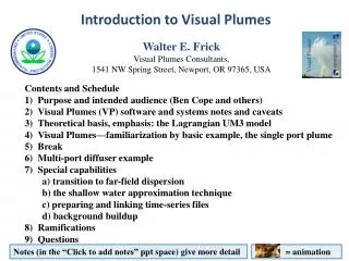
Walter E. Frick Visual Plumes Consultants, 1541 NW Spring Street, Newport, OR 97365, USA Contents and Schedule Purpose and intended audience (Ben Cope and others) Visual Plumes (VP) software and systems notes and caveats Theoretical basis, emphasis: the Lagrangian UM3 model

Introduction to Visual Plumes
E N D
Presentation Transcript
Walter E. Frick • Visual Plumes Consultants, • 1541 NW Spring Street, Newport, OR 97365, USA • Contents and Schedule • Purpose and intended audience (Ben Cope and others) • Visual Plumes (VP) software and systems notes and caveats • Theoretical basis, emphasis: the Lagrangian UM3 model • Visual Plumes—familiarization by basic example, the single port plume • Break • Multi-port diffuser example • Special capabilities • a) transition to far-field dispersion • b) the shallow water approximation technique • c) preparing and linking time-series files • d) background buildup • Ramifications • Questions Introduction to Visual Plumes Abstract = animation EPA Modeling Webinar 22-24 Jan 2013 Notes (in the “Click to add notes” ppt space) give more detail
Visual Plumes, a model platform available through EPA: • CEAM at Athens, Georgia: http://www.epa.gov/ceampubl/ • Manual: http://www.epa.gov/ceampubl/swater/vplume/VP-Manual.pdf • Software and update: http://www.epa.gov/ceampubl/swater/vplume/index.html Software and systems notes and caveats EPA Modeling Webinar 22-24 Jan 2013
Software and update: http://www.epa.gov/ceampubl/swater/vplume/index.html Software and systems: CEAM website Virtual Beach Authors of Ver. 1 (Research) Frick and Ge EPA Modeling Webinar 22-24 Jan 2013
DOS Plumes Visual Plumes • Software Software and systems: install and setup calleableVP external exe’s Project files EPA Modeling Webinar 22-24 Jan 2013
Most of VP: Windows XP and earlier Coding: Delphi 7 (no relation to Windows 7) and earlier 90% interface Dependence on DLLs Borland Database Engine (e.g. BDEinfosetup.exe) After setup:Software and systems: OS and use issues Vista, Windows 7, Windows 8 Users Operating System experience User as novice: most issues can be resolved, not always easily VP Upgrade example: install the BDE somehow; then, open Plumes.exe as Administrator; if vptempstorage error, retry; choose No, start a new project; UM3; if the error recurs, try again EPA Modeling Webinar 22-24 Jan 2013 Notes
Terms and Definitions Aspiration entrainment: tends to be the dominant entrainment mechanism in low currents, including stagnant ambient; in UM3 it is proportional to the area the plume shares with the ambient fluid; where plumes are merged and are demarcated by vertical reflection planes it is assumed that the plume and its neighbor gain and lose equivalent amounts of mass so that no net entrainment occurs across those vertical surfaces, only over the surfaces still exposed to ambient fluid admittedly Background buildup technique: an alternative approach to simulating the effects of merging; plumes are not restricted to the reflection technique but rather act in isolation with the effects of merging accounted for through changes to the plume’s background conditions, particularly the background pollutant concentration; the approach more closely mimics actual mixing mechanisms but, to be rigorous, would involve not only adjusting the background concentration due to the presence of upstream plumes but the physical environment the plume in question occupies, including all variables and velocities Co-flowing plumes: the condition where the effluent discharge and the ambient current flow in the same direction Control volume: the modeling analogue of the plume element in the Eulerian plume model formulation, integral flux equations; unlike the plume element, the model accounts for flux changes as a function of s, the distance along the plume trajectory, the integration step being ds; the stiffness of the model equations requires management of ds that can lead to discontinuous changes in the endpoint dilution as input conditions are changed only incrementally; also sometimes referred to as the plume element, the analogous Lagrangian control volume Counter-flowing plumes: the condition where the effluent discharge flows in the opposite direction of the ambient current Critical Initial Dilution: the flow weighted average of a diffuser plumes’ endpoint dilutions; this review recommends that for the purposes of calculating the CID that merged plumes be treated as grouped entities each with their combined CID Cross-current: ambient current not either co-flowing or counter-flowing will possess a component of velocity that is perpendicular to the plume at the port; cross-currents add another term to the entrainment equations, for example, as in UM3, and will tend to increase overall entrainment in the absence of merging; it is important in reducing the spacing between plumes to values less than the physical spacing Deep-water assumption: integral plume models such as UD and UM3 were developed with the assumption that water depth would not constrain the motion of the plume; the reason for adopting the assumption was to simplify the theory; the models do not plume-water surface interaction; other steps or models must be taken to model the plume beyond the point where any part of it hits the surface (although some relaxation for slightly grazing the surface might be tolerable) Densimetric Froude number: this is a similarity parameter that expresses the relative importance (ratio) of kinetic and potential energy inherent in the plume element at the source; small values represent pure plumes that possess little or no initial velocity (like a heated plate), large values are momentum dominated jets with little or no buoyancy perhaps requiring pump pressure to attain the high velocities; in vertical plumes (like natural draft cooling towers) values less than unity are plumes that possess excess buoyancy to briefly accelerate the plume element at the source causing it to stretch out and dynamically contract its diameter, the analogous mechanism experienced in seawater intrusion; finally, the similarity property allows plumes to be compared across spatial scales, plumes with the same similarity parameters exhibiting the same morphology (plume shape) when plotted in dimensionless terms (for example, in terms of diameters downstream and vertically) DKHw.exe: a version of UDKHDEN that was developed explicitly for use with Visual Plumes (Frick et al. 2004); replaced in this review by an updated version of UDKHDEN (called UD) after DKHw was found to exhibit spurious density behavior in isolated instances and its further use was suspended Effective dilution: effective dilution is the ratio of effluent concentration to plume element concentration, particularly plume element concentration at an endpoint condition; when the ambient concentration is zero the effective dilution is equal to the volume dilution, or more correctly, the mass dilution; judged from an environmental perspective, as opposed to a mechanical mixing perspective, the effective dilution is a better measure of plume performance than volume dilution Effective spacing: is the spacing between centerlines of plumes measured perpendiculat to their trajectories at given points; in terms of the mathematics of the plume model, it continuously estimates the separation between the vertical reflection planes used to constrain the plume element to its allotment of space Endpoint criterion: Initial Dilution models usually report when significant conditions are met, for example trapping level, maximum rise, merging, and surface hit; these conditions can serve as endpoint markers, or criteria, for modeling or regulatory purposes Endpoint dilution: the dilution corresponding to some regulatory or modeling criterion for determining diffuser performance, like the trapping level, maximum rise, or surface hit condition Entrainment: discharged plumes are usually energetic, possessing kinetic energy (great velocity or momentum) and potential energy of buoyancy that converts into kinetic energy along the plume trajectory; through the Bernoulli effect the plume shear velocity aspirates, or entrains, ambient fluid into the plume; ambient water delivered at the plume boundary by current is also entrained by virtue of the turbulence in the plume Far-field: when using integral models such as UD and UM3 the modeling domain is often divided into near-field and far-field subdomains; far-field dispersion is dominated by ambient passive diffusion processes and the rate of dilution is comparatively small; in VP the Brooks far-field algorithm may be used to estimate additional plume dilution Forced entrainment: tends to be the dominant entrainment mechanism in moderate and high currents; in UM3 it is proportional to the area the plume projects to the current and is developed using the Projected Area Entrainment Hypothesis; where plumes are merged and are demarcated by vertical reflection planes it is assumed that the plume and its neighbor gain and lose equivalent amounts of mass so that no net entrainment occurs across those vertical surfaces, only over the surfaces still exposed to ambient fluid Grouped plumes: plumes that fully merge into a single entity as would be seen by an observer located at the downstream mixing zone boundary; the CID of grouped plumes would be based on the product of a single joint representative initial dilution and the combined flow of all contributing plumes Guidelines: the Puerto Rico EQB April 1988 interim guidelines—Mixing Zone and Bioassay Guidelines Half-spacing technique: a simplifying technique to simulate cross-diffuser merging the basic assumption being that counter-flowing plumes will flow across the diffuser and merge with the co-flowing plumes on the other side and will do so achieving about the same mass or volume dilution; seen at some distance downstream, as at the mixing zone boundary, the coflowing and counterflowing plumes’ details are considered relatively unimportant and it appears as if two plumes at half the spacing are issued from downstream side of the diffuser; used in lieu of the more rigorous background buildup technique Initial dilution: the plume dilution that results from the action of internal plume turbulence; the turbulence arises from velocity shear between the plume and the ambient; plume velocity, or momentum, is provided at the source and maintained to greater or lesser extent by the conversion of buoyancy into vertical velocity; experiments show that plume turbulence generally “collapses” near, but beyond, the point of maximum rise, hence it is often used as the endpoint for the initial dilution process Isolated plumes: either plumes from single port discharges or plume from multiport discharges that do not interact with other plumes; the definition can be troublesome when plumes do not merge in their near-field regions but a far-field portion of the upstream plume recirculates and interacts with the downstream plume in its near-field, then the downstream plume cannot be considered to be isolated and merging techniques should be considered Lmz, mixing zone length scale: for both UD and UM3 simulations Visual Plumes can display the trajectory of a plume and the plume boundaries, i.e. its variable diameter, in plan view, i.e., as if on a map; given the coordinates are provided, VP can also display the configuration of the diffuser, like the diffuser axis; Lmz is the distance between outermost end of the diameter drawn perpendicular to the plume trajectory at the endpoint dilution and the nearest point on the diffuser axis, i.e. perpendicular to the diffuser axis Maximum rise: the greatest rise of buoyant plumes in density stratified medium often considered to be the end of the initial dilution region, thus an endpoint criterion Merging plumes: many discharges involve multiple plumes issuing from submerged diffusers; depending on the spacing between them, these plumes will generally interact with each other either in the initial dilution or the far-field region; Initial Dilution models such as DKHDEN and UM3 were originally developed around single plumes discharged to deep water and use the reflection technique to estimate the effects of merging on dilution Near-field: when using integral models such as UD and UM3 the modeling domain is often divided into near-field and far-field subdomains; the near-field is the region in which initial dilution occurs and the plume element moves from source to maximum rise, other endpoint criteria not encountered; the energy of the plume is the primary generator of internal turbulence that serves to entrain ambient fluid Normal: used synonymously with perpendicular Perpendicular: used synonymously with normal or normal to Physical spacing: at its most elemental is the physical distance between neighboring ports as from port centerline to centerline; the physical spacing, the diffuser geometry, the current angle, and the merging technique together determine the spacing that defines the separation between plume centerlines at different points along the trajectory Plume element: in the Lagrangian framework on which UM3 is based the plume element is initially defined to be a right cylinder with the diameter of the port or vena contracta and an arbitrary but small height, h; a fundamental axiom of the model is that all mass originally in the plume element remains in the plume element even as it grows from entrainment and moves along its trajectory; the steady state assumption allows h to be computed at any point and forms the basis for the “jelly sandwich” equation (redistribution of mass normal to the plume axis); in general, the plume element takes on the shape of a circular wedge with its faces normal to the plume axis; the independent variable is time and quantities such as the amount of entrainment are computed in small time steps; the term plume element may also include the analogous concept of the control volume Projected area: the apparent area of the plume element seen by an observer sighting along the direction of the current approaching the plume; the mathematical projection of the plume element onto a vertical plane normal to the current direction; the total area projected by the entire plume onto a vertical plane normal to the current direction; the total forced entrainment would be proportional to the total projected area excluding area above the water surface Quarter-spacing technique: a simplifying technique to simultaneously simulate cross-diffuser and cross-leg merging in wye diffuser configuration where the plumes from the upstream leg are believed to flow into and merge with plumes of the downstream leg; seen at some distance downstream, as at the most downstream mixing zone boundary, the coflowing and counterflowing plumes’ details are considered relatively unimportant and it appears as if four plumes at quarter spacing are issued from downstream side of the downstream leg of the diffuser; often used in lieu of the more rigorous background buildup technique Reflection technique: at their common boundaries merging plumes entrain each other, one’s diameter intrudes into the body of the other, and vice versa; any mass common to two entities requires careful accounting for mass to assure there is not double accounting; the reflection technique provides imaginary vertical planes between plumes that assure the conservation of mass; each plume is allotted its own space into which to develop; both entrainment and growth must occur at the remaining free surface the plume shares with the ambient fluid Spacing distance: the spacing between plumes determines how much of the plumes trajectory is subject to plume merging; measured horizontally perpendicular to the plume centerline trajectory, merging begins when the plume diameter becomes larger than the spacing distance; in general, the spacing distance varies along the plume trajectory because the plume trajectory will bend into cross-currents and therefore identical trajectories from neighboring plumes spacing distance will be a function of where the plume element is along the trajectory at the time of interest Steady state: an important assumption that makes the mathematical formulation of entrainment models tractable; steady state implies the morphology, or shape or envelope, of the plumes are invariant in time; successive releases of effluent (the initial control volume or plume element) perform the same motions as they flow through the stationary envelope from discharge to maximum rise (and beyond); in UM3 the assumption makes it possible to calculate the length of the plume element at any point along the trajectory, that, coupled with the change in mass during the time step and the equation of state, allows the plume diameter to be computed at any point; steady state also indirectly determines the spacing between plumes Surface hit criterion: entrainment is a plume surface phenomenon, when plume boundaries reach the surface the plume area available to entrainment is reduced or cut off and the underlying model assumptions are no longer satisfied in the way the model was developed; to be conservative the criterion should be considered to be an endpoint condition for initial dilution Trapping level: the depth at which the plume control volume or plume element possesses the same density as the ambient fluid at that depth; in many instances the plume continues to develop beyond this point, ultimately reaching its maximum rise or the surface water depth and density stratification permitting; in the early days of modeling this was the most popular modeling endpoint but most modelers agree that maximum rise or surface hit are the important endpoints in determining initial dilution UD: the most recent version of the DKHDEN three-dimensional Eulerian integral flux plume model; a subroutine has been written for Visual Plumes to read and interpret UD output, providing information of the plume boundary surface hit condition and set up with an estimate of the reduced spacing when run from VP UDKHDEN: a three-dimensional Eulerian integral flux plume model; a version, DKHw, was developed to run in Visual Plumes; a 2011 updated version UD is used herein; other models include UM3, a Lagrangian model, and NRFIELD, an empirical model of multi-port diffusers; UM3 is developed around the concept of the plume element UM3: a three-dimensional Lagrangian plume model found in Visual Plumes, other models include DKHw, an Eulerian integral flux model, and Nearfield, an empirical model of multi-port diffusers; UM3 is developed around the concept of the plume element Vena contracta: the minimum area cross-section in the fluid stream discharging from a port or any orifice; the area and velocity at that point are used to help define the initial conditions for model input Visual Plumes: the EPA platform for running several plume models in common, including UD, UM3, and NRFIELD Volume dilution: the common quantity used to characterize the effectiveness of a diffuser; the problem with volume dilution is that often it does not differentiate between water volume entrained from the prevailing ambient fluid and water volume representing entrained plume fluid; the half and quarter spacing techniques normally would guard against misuse of volume dilution but, with wye diffusers, generally the half-spacing technique alone would not; effective dilution avoids the pitfalls of volume dilution and represents the mass balance of both effluent and entrained sources Wastefield width and merging: one way to better estimate the effects of merging plumes issued from a cluster of sources is to run the individual plumes in the context of the current speed and direction (plan view geometry) to estimate the wastefield width and use that information to estimate the effective reduced spacing, and, finally, rerun the plumes with the reduced spacing to obtain a final estimate of the initial dilution Worst case conditions: as a substitute for a lack of ambient measurements or to simplify the process of modeling all possible conditions and analyzing the results statistically, worst case conditions may be developed that will provide a conservative initial dilution estimate when used as input conditions to the model of choice; worst case conditions are often limited to a low current speed (like ten percentile) and a stable ambient density (or salinity and temperature) stratification; for merging plumes this approach should be expanded to include current direction, as co-flowing plumes will generally not represent the worst case Terms and definitions Reference material (also, when slides are viewed in Powerpoint, check for additional notes) EPA Modeling Webinar 22-24 Jan 2013 Notes
Recommended Tutorial Get the VP manual!! Tutorial starts on page 4.7 to 4.20 EPA Modeling Webinar 22-24 Jan 2013
Visual Plumes Manager/ Model Platform VP’s main tab: the Diffuser tab
Example r-click pop-up menu EPA Modeling Webinar 22-24 Jan 2013
DKHW: Physics-based exe, Eulerian numerical formulation, integral flux model. One or multi-port diffusers. NRFIELD: Empirical, dimensional analysis and curves fit to data; exe. Based on T-risers, for 4 or more ports. Visual Plumes Model Suite UM3: Physics-based native, Lagrangian numerical formulation, material element model. One or multi-port diffusers. el PDS: Eulerian integral flux surface plume model; exe. Buoyant discharges DOS Plumes: predecessor of Visual Plumes, runs RSB (pre-NRFIELD) and UM (Updated Merge model; pre-UM3). Features auto cell-fill: displays similarity parameters, length scales, cormix classes. Dreamware prototype depicts wire-mesh graphics, like UM3, vector based. All but PDS link to the Brooks far-field algorithm, far-field dispersion model. EPA Modeling Webinar 22-24 Jan 2013 Notes
There is more to follow on empirical, hydrodynamic fluid dynamic codes, empirical, Eulerian integral flux and Lagrangian plume models. explain illustrate “demystify“ touch on basic principles of physics mathematical formulations modeling assumptions UM3 examples (built into Visual Plumes--not an external application) examples chosen for simplicity, generality, and teaching potential More to come VP is public domain software EPA Modeling Webinar 22-24 Jan 2013
What’s the answer? What’s the answer? Mixing Zone analysis World What’s the answer? Client Here are THREE 3-) VP: dkh, nfd, um3… User Answers, yes, but no one knows it all (otherwise there’d one). MZ analysis is a partnership EPA Modeling Webinar 22-24 Jan 2013
Whom to believe, best? How feasible? The problem/model universe Problem domain Visjet… TOE VP Cormix VP is public domain software Everyone can be on the same page Facilitates inter-model comparison & competition EPA Modeling Webinar 22-24 Jan 2013
Before illustrating by example: Let us take a brief tour of plume problem, physics, and prediction Touch on: capabilities limitations pitfalls mystery and ambiguity And end with promise: A bonus rule Reason for optimism and confidence Mixing effluent in environment—basic science EPA Modeling Webinar 22-24 Jan 2013 Notes
Conceptual model in a snapshot:it’s air but, by similarity, it could be water Some questions: Current? Steady? Cross-section round? Jet or plume? Phase changes? Ambient stratification? Dimension imply dilution? source plume Receptor (somewhere) other plumes EPA Modeling Webinar 22-24 Jan 2013
Theory of Everything • “A theory of everything (ToE) or final theory is a putative theory of theoretical physics that fully explains and links together all known physical phenomena, and predicts the outcome of any experiment that could be carried out in principle.” • http://en.wikipedia.org/wiki/Theory_of_everything • In plume modeling this dream is called Computational Fluid Dynamics (CFD). In principle a comprehensive CFD model could model any plume in relationship to other plumes and their bathymetric, chemical, and physical environments. All that is required is precise and accurate knowledge of • Initial conditions (IC) • Boundary conditions (BC) • Forcing functions • Chemistry • Physics • Thermodynamics…. Why not the TOE for Visual Plumes? EPA Modeling Webinar 22-24 Jan 2013
Meet a CFD model: grid and input Model tidal forcing Model tidal forcing River flow FVCOM unstructured model grid Zooming would reveal fine structure, sources, etc. Wind Notes
CFD model output: salinity animation Points to watch 1) Lake Pont. outflow 2) river plume length 20 km Discharge from Lake Pontchartrain after Katrina Courtesy Tarang Khangaonkar et al., 2005 Notes hrs
Zooming in a little Discharge from Lake Pontchartrain after Katrina Courtesy Tarang Khangaonkar et al., 2005 Notes hrs
In theory, we can accurately model plumes using accurate CFD models. • However, consider the • Resources • Setup • Data collection (IC, BC….) • Expense…. • We (modelers, users…) must formulate dispersion coefficients everywhere (eddies and turbulence) (models in themselves) • A dream for most of us. On to Visual Plumes’ imperfect answers. Done! Except…. EPA Modeling Webinar 22-24 Jan 2013
While we wait for CFD, how about going to the laboratory for solutions? Empirical models. • Visual Plumes comes bundled with an older version of the NRFIELD empirical model. (This is essentially the Roberts, Snyder, Baumgartner model, RSB, found in DOS Plumes.) NRFIELD is a stand-alone executable that can be called by VP: • VP creates the input file • VP initiates NRFIELD execution • VP reads the output file and displays output • Considerations: • NRFIELD addresses multiple merging plume problems • It is an endpoint model… One alternative: empirical modeling EPA Modeling Webinar 22-24 Jan 2013 Notes
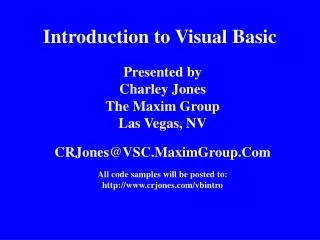
A dense plume The “plume envelope” or plume boundary maintains a steady appearance Evidence of detraining fluid A household dehumidifier plume showing evidence of unexpected behavior. Mimicking the laboratory, will NRFIELD be the first model modified to explain observations? EPA Modeling Webinar 22-24 Jan 2013
UM3 dense plumes Focus on rise and impact point. Red: aspiration coefficient the standard 0.10; blue: 0.05. EPA Modeling Webinar 22-24 Jan 2013
Eulerian integral flux models VP example: DKHW or UDKHDEN Differential equations Physics of mass, momentum, energy… Integrating factor: ds Flux balances over control volumesfixed in space Steady state assumed EPA Modeling Webinar 22-24 Jan 2013 Notes
Unstratified buoyant jet in the labConceptual morphing We see evidence of steady state, time-averaging, plume morphology (round plume assumption)… Notes
How does numerical Eulerian method work? Derive (compute)… density buoyancy area… mass flux momentum flux energy flux … Define the source: IC, BC.. velocity vector radius temperature salinity concentration current orientation... ( )s+Δs = ( )s + EΔs By the way, the integral is the mass flux Define coordinate system and location z Δs y x
An Eulerian simulation“stacking” the control volumes trajectory distance s An Eulerian control volume volume “frames” are stationary mass enters right mass enters around edge (entrainment) mass exits left ds (or Δs) ̴̴ 1.0 port dia Mass flux increases EPA Modeling Webinar 22-24 Jan 2013 Notes
As the fluid entering the bottom of the control volume, augmented by the entrained fluid coming in from the ambient, all exits the top of the control volume we may ask: • At some travel distance s, is dilution approximately directly proportional to the area of the cross-section of the plume? • Yes or no? • Other than holding the plume shape constant, the significance of steady state is a little obscure (implicit?) with Eulerian models. Does it help answer the question? More to follow. Any handy laws/rules on dilution? EPA Modeling Webinar 22-24 Jan 2013 Notes
We just saw the Eulerian integral flux formulation The infinitesimal distance ds is the integrating factor Differential equations express fluid dynamics (physics) e.g. conservation of mass: where the integral is consistent with the choice of control volume In finite difference models ds is expressed by , which is small Other equations, e.g. eqn. of state, bookkeeping,… round out the model Finite difference plume model comparison With the Lagrangian integral flux formulation we will find The infinitesimal time dt is the integrating factor The control volume is called the plume element It is a material (coherent) element Again, differential equations express fluid dynamics (physics) e.g. conservation of mass: where In finite difference models dt is expressed by , which is small Again, other equations, e.g. eqn. of state, bookkeeping,… round out the model EPA Modeling Webinar 22-24 Jan 2013 Notes
Eulerian plume models came first (Fan 1967, Weil 1974….) Late to the party, when Winiarski & Frick developed the Lagrangian plume model formulation they set out to prove its equivalence to the Eulerian formulation This was successful given the same assumptions: a round plume, steady state, equations of state,…. The proof was published and clarified the initial conditions of Weil’s Eulerian plume model integration (upper and middle traces). Replication: proving the Lagrangian model EPA Modeling Webinar 22-24 Jan 2013 Notes
Two cars stopped, after they start how far apart are they when they reach the open road traveling, say, 60mph (88fps)? • Car 2 • Car 1!! • Car 2 steady state leads to bonus ? answer • Car 1 • Trick question, we don’t know the answer. However, we would if (1) we knew the time between Car 1 and Car 2 starting, and, • (2) both drivers drove identically (same time history, steady state). • E.g., if they started 1.00sec apart, they would always be 1.00sec apart, which translates to 88ft at 60mph, 44ft at 30mph, etc. EPA Modeling Webinar 22-24 Jan 2013 Notes
Lagrangian plume element Lagrangian material elements trace through time, all contain the same effluent they had at age 0 Here, dt = tlead – ttrail= 4sec Element age (r to l): 0, 4, 24, 44, 64, and 94 sec Cross-section round…. Length (h) is variable, WHY? h(t=24) h(t=4) h(t=0) EPA Modeling Webinar 22-24 Jan 2013 Notes
Eulerianpl Steady state and plume element length, h;the “free” equation gives the answer The mass of the plume element or Thus r is not only a function of the mass of the plume element but also its height (or length) h The answer to the poll question is NO EPA Modeling Webinar 22-24 Jan 2013 Notes
Corollaries (bonuses) A plume discharged to high current will be thin (Dye studies in high current areas will have trouble finding the plume) A plume discharged to low current will be fat, surface hit issues The “free” equation completes the equivalence with the Eulerian formulation Explicit with UM3, these truths are implicit in the Eulerian models EPA Modeling Webinar 22-24 Jan 2013
Define boundary conditions (BC): ambient properties (temperature T, salinity, current, concentration, decay), stratification of properties Define initial conditions (IC): element mass m, properties (temperature T, salinity, time, position…), radius r, and, of course, h (or ho) and Δt UM3 skeleton or flow chart Begin model loop Bookkeeping: interpret and interpolate the ambient array of properties Calculate Δm, the mass entrained into the plume element in the time step Δt. Requires an entrainment function Calculate new element properties by mixing m and Δm. E.g., new salinity: Apply equation of state (, S, T); calculate dynamics: momentum, energy, buoyancy; calculate displacement (new position) Use the “free” eqn. (h) (steady state) to solve for radius: More bookkeeping, like output. Finally, return to the beginning of the model loop EPA Modeling Webinar 22-24 Jan 2013
Considering that identical assumptions result in Eulerian integral flux and Lagrangian model equivalence, what sets integral models apart are the assumptions (if the underlying assumptions are different) • entrainment hypotheses (functions) • numerical convergence scheme • ancillary capabilities like plume merging and treatment of surfaces • Facilities: unit conversion, time-series input, and other capabilities or constraints • Given the assessment satisfies the underlying assumptions used in model development (viz. deep water and steady state) the entrainment functions deserve the greatest attention. The name of the game: entrainment EPA Modeling Webinar 22-24 Jan 2013
Early entrainment conception historical context a) forced entrainment due to current (more next 3 slides) b) aspiration entrainment due to suction: this mechanism is due to the Bernoulli effect; the inflow velocity is proportional to the surface area of the element and the velocity shear between the average plume element velocity and the ambient velocity; it is governed by an adjustable aspiration entrainment coefficient EPA Modeling Webinar 22-24 Jan 2013
Projected Area Entrainment (PAE) Perspective and three orthogonal views of the plume element as conceived in UM3 (in a. it’s the area of the ring) The PAE hypothesis postulates forced entrainment = (ambient density)*( current)*(total area projected to the current) Total projected area of the plume element (3D conception) = (a) growth + (b) cross-flow+ (c) cylinder and curvature The PAE hypothesis appears to require no adjustment; the coefficient is 1.0. EPA Modeling Webinar 22-24 Jan 2013
Before recognizing the significance of steady state (aka jse) • Developing the Lagrangian “pre-UM3” from scratch took about a year. • ?About how many entrainment assumptions/hypotheses did W&F try in the effort to obtain good fit to Fan’s data? • 1, 2, 5, 10, 20, 50? • ?After adding the “free” equation for plume element length, how many revisions before formulating the forced entrainment equation as a function of r, h, and θ? • 1, 2, 5, 10? Follow science for the answer--yes, but… EPA Modeling Webinar 22-24 Jan 2013 Notes
Dream model element & entrainment • Wedge shape and overlap (left) • The concept of all approaching ambient fluid being captured by the plume element (middle and right) Notes
Differential equations (DE) express changes with time or distance that cannot be solved exactly (analytically). Solving stiff equations means, in UM3, a new Δt= t2 – t1 each step UM3: Δtchanges gradually & smoothly DKH: Δs changes relatively larger 2.5” ports Model convergence scheme discontinuity 3.5” ports Figure: Two diffuser sections. Each of the 6 dilution estimates correspond to port spacing varying from 3.66 to 3.565m, very little. Between 3.570 and 3.565m the predicted DKH dilution increases over 8%. Which side of the discontinuity has the more accurate solution? EPA Modeling Webinar 22-24 Jan 2013 Notes
Model comparison example: 1-port Fan Run 16 input; DKHW (blue) and UM3 (red) simulations. Stagnant, density stratified environment.
VP verification example Same input as previous slide. VP allows input from text files, a capability used to show the experimental plume trace.
Example UM3 verification Six center panels, UMERGE (UM3 predecessor) model predictions. Schatzmann’s multi-parameter model predictions in margins. Data from Fan, 1967.
Preface to the live demonstration EPA Modeling Webinar 22-24 Jan 2013
menus, buttons Fan 16 diffuser tab Active tabs Project title set tab jump configure models Ambient file list (one shown, r-click menu) space for project notes run scheme selected model adjust units click unit for menu selected case and input diffuser table show parameters click in time-series files