Atomic Structure: A Journey into the Microscopic World
Explore the intricate world of atomic structure, from John Dalton's three particle model to J.J. Thomson and Robert Millikan's groundbreaking charge measurements. Learn how atoms form compounds and the significant experiments that unraveled the mysteries of the atom. Discover key insights and controversies in the history of atomic research.

Atomic Structure: A Journey into the Microscopic World
E N D
Presentation Transcript
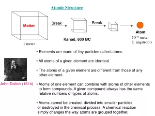
Atomic Structure Break Break Matter Atom 10-10 meter (1 angstrom) Kanad, 600 BC 1 meter • Elements are made of tiny particles called atoms. • All atoms of a given element are identical. • The atoms of a given element are different from those of any • other element. • Atoms of one element can combine with atoms of other elements • to form compounds. A given compound always has the same • relative numbers of types of atoms. • . • Atoms cannot be created, divided into smaller particles, • or destroyed in the chemical process. A chemical reaction • simply changes the way atoms are grouped together. John Dalton (1814)
Atoms are made up of 3 types of particles: Electrons Protons (It is 1840 times heavier than an electron) Neutrons (Similar mass as that of a proton) These particles have different properties. Electrons are tiny, very light particles and have negative electrical charges (-). Protons are much larger and heavier than electrons and have the opposite charges, A proton has a positive (+) charge. Neutrons are large and heavy like protons, however neutrons have no electrical charge. A Hydrogen Atom
Determination of the Charge on an Electron J.J.Thomson H.A. Wilson J.S.E. Townsend The charge on electron was first measured by J.J. Thomson and two co-workers (J.S.E. Townsend and H.A. Wilson), starting in 1897. Each used a slightly different method. Townsend's work depended on the fact that drops of water will grow around ions in humid air. Under the influence of gravity, the drop would fall, accelerating until it hit a constant speed. He determined the e/m ratio of the droplets, then multiplied by the mass of one droplet to get the value for e. Thomson, Townsend, and Wilson each obtained roughly the same value for the charge on positive and negative ions. It was about 1 x 10-19 coulombs. This work continued until about 1901 or 1902.
Robert A. Millikan's Measurement Robert A. Millikan started his work on electron charge in 1906 and continued for seven years. His 1913 article announcing the determination of the electron's charge is a classic and Millikan received the Nobel Prize for his efforts. The actual apparatus used in the Oil-Drop experiment by Millikan
Some points about the experiment : 1. The two plates were 16 mm across, "correct to about .01 mm."2. The hole bored in the top plate was very small.3. The space between the plates was illuminated with a powerful beam of light.4. He sprayed oil ("the highest grade of clock oil") with an atomizer that made drops one ten-thousandth of an inch in diameter.5. One drop of oil would make it through the hole.6. The plates were charged with 5,000 volts.7. It took a drop with no charge about 30 seconds to fall across the opening between the plates.8. He exposed the droplet to radiation while it was falling, which stripped electrons off.9. The droplet would slow in its fall. The drops were too small to see. What he saw was a shining point of light.10. By adjusting the current, he could freeze the drop in place and hold it there for hours. He could also make the drop move up and down many times.11. Since the rate of ascent (or descent) was critical, he has a highly accurate scale inscribed onto the telescope used for droplet observation and he used a highly accurate clock, "which read to 0.002 second
Millikan's Improvements over Thomson • 1. Oil evaporated much slower than water, so the drops stayed essentially constant in mass. • 2.Millikan could study one drop at a time, rather than a whole cloud. • 3.In following the oil drop over many ascents and descents, he could measure the drop as it lost or gained electrons, sometimes only one at a time. Every time the drop gained or lost charge, it ALWAYS did so in a whole number multiple of the same charge. • The value as of 1991 (for the charge on the electron) is 1.60217733 (49) x 10¯19 coulombs. This is less than 1% higher than the value obtained by Millikan in 1913. The 49 in parenthesis shows the plus/minus range of the last two digits (the 33). It is unlikely that there will be much improvement of the accuracy in years to come.
Interesting Fact about Robert Millikan's Experiment In "The Discovery of Subatomic Particles" by Steven Weinberg there appears a footnote on p. 97. It reads: . . . . there appeared a remarkable posthumous memoir that throws some doubt on Millikan's leading role in these experiments. Harvey Fletcher (1884-1981), who was a graduate student at the University of Chicago, at Millikan's suggestion worked on the measurement of electronic charge for his doctoral thesis, and co-authored some of the early papers on this subject with Millikan. Fletcher left a manuscript with a friend with instructions that it be published after his death; the manuscript was published in Physics Today, June 1982, page 43. In it, Fletcher claims that he was the first to do the experiment with oil drops, was the first to measure charges on single droplets, and may have been the first to suggest the use of oil. According to Fletcher, he had expected to be co-author with Millikan on the crucial first article announcing the measurement of the electronic charge, but was talked out of this by Millikan.
Electron Spin Two types of experimental evidence which arose in the 1920s suggested an additional property of the electron. One was the closely spaced splitting of the hydrogen spectral lines, called fine structure. The other was the Stern-Gerlach experiment which showed in 1922 that a beam of silver atoms directed through an inhomogeneous magnetic field would be forced into two beams. Both of these experimental situations were consistent with the possession of an intrinsic angular momentum and a magnetic moment by individual electrons. Classically this could occur if the electron were a spinning ball of charge, and this property was called electron spin. An electron spin s = 1/2 is an intrinsic property of electrons. Electrons have intrinsic angular momentum characterized by quantum number 1/2. In the pattern of other quantized angular momenta, this gives total angular momentum The resulting fine structure which is observed corresponds to two possibilities for the z-component of the angular momentum. This causes an energy splitting because of the magnetic moment of the electron.
A Helium Atom Ions • Ions are formed by addition or removal of electrons from neutral atoms. • Cations (removal of electrons from atoms). • Anions (addition of electrons to atoms). H+ cation H-atom H- anion
Isotopes • Two atoms with different numbers of neutrons are called isotopes. • For example, an isotope of hydrogen exists in which the atom contains • 1 neutron (commonly called deuterium). Hydrogen Atomic Mass = 1 Atomic Number = 1 Deuterium Atomic Mass = 2 Atomic Number = 1 Since the atomic mass is the number of protons plus neutrons, two isotopes of an element will have different atomic masses (however the atomic number, Z, will remain the same).
Plum Pudding Model By 1911 the components of the atom had been discovered. The atom consisted of subatomic particles called protons and electrons. However, it was not clear how these protons and electrons were arranged within the atom. J.J. Thomson suggested the "plum pudding" model. In this model the electrons and protons are uniformly mixed throughout the atom:
Rutherford's Planetary Modelof the Atom Rutherford tested Thomson's hypothesis by devising his "gold foil" experiment. Rutherford reasoned that if Thomson's model was correct then the mass of the atom was spread out throughout the atom. Then, if he shot high velocity alpha particles (helium nuclei) at an atom then there would be very little to deflect the alpha particles. He decided to test this with a thin film of gold atoms. As expected, most alpha particles went right through the gold foil but to his amazement a few alpha particles rebounded almost directly backwards.
These deflections were not consistent with Thomson's model. Rutherford was forced to discard the Plum Pudding model and reasoned that the only way the alpha particles could be deflected backwards was if most of the mass in an atom was concentrated in a nucleus. He thus developed the planetary model of the atom which put all the protons in the nucleus and the electrons orbited around the nucleus like planets around the sun.
Limitations of Rutherford Model There appeared something terribly wrong with Rutherford's model of the atom. The theory of electricity and magnetism predicted that opposite charges attract each other and the electrons should gradually lose energy and spiral inward. Moreover, physicists reasoned that the atoms should give off a rainbow of colors as they do so. But no experiment could verify this rainbow. In 1912 a Danish physicist, Niels Bohr came up with a theory that said the electrons do not spiral into the nucleus and came up with some rules for what does happen. (This began a new approach to science because for the first time rules had to fit the observation regardless of how they conflicted with the theories of the time.)
Atomic Spectra • When one heats up a gas, it emits light of various wavelengths. • The simplest spectrum is that for a Hydrogen atom. • The spectrum of hydrogen is particularly important in astronomy • because most of the Universe is made of hydrogen. • In 1885, Balmer discovered emission of H-atom in the visible region. • The Balmer Series involves transitions starting (for absorption) • or ending (for emission) with the first excited state of hydrogen. • Soon, the Lyman Series was discovered that involves transitions • which start or end with the ground state of hydrogen(UV region)
By 1913, many more series were known: Paschen (Near Infrared), • Brackett (Far Infrared). Rydberg proposed an experimental data to fit this: = 1/λ= R (1/m2-1/n2) R=Rydberg constant (109677 cm-1) m,n= integers n m Series Region UV Visible Near-IR Far-IR 1 2 3 4 2,3,4,.. 3,4,5,… 4,5,6,… 5,6,7,… Lyman Balmer Paschen Brackett
The Bohr Model (1913) 1. The orbiting electrons existed in orbits that had discrete quantized energies. That is, not every orbit is possible but only certain specific ones. 2. When electrons make the jump from one allowed orbit to another, the energy difference is carried off (or supplied) by a single quantum of light (called a photon) which has an energy equal to the energy difference between the two orbitals. 3. The allowed orbits depend on quantized (discrete) values of orbital angular momentum, (L) according to the equation: n= principle quantum number, 1,2,3… h=Planck’s constant
The energy of electron with a principle quantum number, n: Now, we can derive the energy required for transition from an nth level to the mth level as: 1/λ = meqe4/8ch3ε0(1/m2-1/n2) Same as R=Rydberg constant (109677 cm-1) Atoms possess shells in which only a fixed number of electrons can be accomodated: K=2,L=8,M=8,N=8
Wave-Particle Duality Wave-particle duality states that a particle such as an electron must also have wave properties such as wavelength. In order to maintain a stable orbit, the electron should have an integral number of wavelengths in its travels around the nucleus. If the wavelengths do not match going around the circle, destructive interference between the wavelengths causes the waves to disappear. This observation led scientists to describe electron motion using equations for wave motion. Electron +
deBroglie relationship (1924) • In 1924, Louis-Victor de Broglie formulated the de Broglie hypothesis, • claiming that all matter has a wave-like nature; he related wavelength, • λ (lambda), and momentum, p: • λ=h/p What is the wavelength of an electron that has a velocity of 5.94×108 cm/sec (electron accelerated through 100V) . What is the wavelength of a man (70 Kg) walking at a velocity of 10km/hour. Why don’t we have waves around us? 2005 Fullerene is the largest object known till now that has an observable wavelength (λ = 2.5 picometer) C60
Uncertainty principle (1927) "The more precisely the POSITION is determined,the less precisely the MOMENTUM is known" The most common one is the uncertainty relation between position and momentum of a particle in space: Thus, for small particles like electrons or photons, it is not possible to determine both the position and the momentum simultaneously with the same accuracy. This uncertainty leads to some strange effects. For example, in a Quantum Mechanical world, I cannot predict where a particle will be with 100 % certainty. I can only speak in terms of probabilities. For example, I can only say that an atom will be at some location with a 99 % probability, and that there will be a 1 % probability it will be somewhere else (in fact, there will be a small but finite probabilty that it can even be found across the Universe). This is strange and very different from the macroscopic world that we live in.
Failure of the Bohr’s Model: • Consider an electron which has a mass of 9.1× 10⁻³¹Kg • Let the electron be moving in the 1st Bohr orbit (radius=0.52 Å) in the hydrogen atom. • It will have a momentum of 2×10-21 Kg cm/sec. • To know this momentum within 1% accuracy, the uncertainty in momentum has to be • smaller than 2×10-23 Kg cm/sec. • Then Δx will be 330 Å !! This is ~300 times the diameter of the 1st Bohr radius. • You cannot even say that the electron was within the atom at all ! Bohr’s shells become most probable position regions (orbitals) in Quantum Mechanics
Hydrogen Atom Potential We will solve Schrodinger equation for an electron bound to an proton by electromagnetic potential to make one hydrogen atom. 3-D Schrodinger equation : : Where, Here is called Laplacian. Here tha Laplacian is in Cartesian coordinate. So,
So, Laplacian in Spherical coordinates, So, Schrodinger equation in Spherical coordinates,
Separation of Variables Now we can solve each of these two equations separately
Solution for part For the case of m = 0 Putting these values in the above equation,
Power Series Solution Plug into, To find, P(x) diverges at x = 1
Solution of Radial Part Solution of these equations under the constraints placed on the wavefunction leads to series solutions in the form of polynomials called the associated Laguerre functions. In order to fit the physical boundary conditions, these solutions contain a parameter n which can take only positive integer values; this parameter is called the principal quantum number. The form of the radial solutions is Where Ln,l is the associated Laguerre function. The first few radial wavefunctions R are shown as part of the hydrogen wavefunctions The principal quantum number or total quantum number n arises from the solution of the radial part of the Schrodinger equation for the hydrogen atom. The bound state energies of the electron in the hydrogen atom are given by
The normalized position wavefunctions, given in spherical coordinates are: Where, And a0 is Bohr Radius Are Generalized Laguerre Polynomyals Yl,m( θ,φ ) Is a spherical harmonics
Probability densities for the electron at different quantum numbers (l)
Electronic Configuration of atoms The electron configuration is the arrangement of electrons in an atom. The electrons occupy specific probability regions, who's shapes and electron capacity are denoted by the letters s,p,d,f. s-orbital p-orbital d-orbital
There are four quantum numbers: • Principal Quantum Number (n): This has range from 1 to n. This represents • the total energy of the system (Do you remember the Bohr’s energy expression). • Azimuthul Quantum Number (l): This has range from 0 to n-1. This is related • to the orbital angular momemtum. • Magnetic Quantum Number (m): This has a range from –l to +l. This determines • energy shift of an atomic orbital due to external magnetic field (Zeeman effect). • Spin Quantum Number (s): It takes values of +½ or -½ (sometimes called "up" • and "down"). The electron not only rotates around the nucleus also rotates (spins) around itself.
Origin of Magnetic Quantum Number For l = 2 Precession of the angular momentum vector about the -axis, defined by a magnetic field. Space Quantisation of angular momentum of electron for l = 2
Pauli exclusion principle No two electrons in one atom can have the same set of these four quantum numbers Start filling the electrons
s-block atoms (have valence electrons in s-orbitals) p-block atoms (have valence electrons in p-orbitals) d-block atoms (have valence electrons in d-orbitals) f-block atoms (have valence electrons in f-orbitals)
Exceptions: d subshell that is half-filled or full (ie 5 or 10 electrons) is more stable than the s subshell of the next shell. instance, copper (atomic number 29) has a configuration of [Ar]4s1 3d10, not [Ar]4s2 3d9 as one would expect by the Aufbau principle. Likewise, chromium (atomic number 24) has a configuration of [Ar]4s1 3d5, not [Ar]4s2 3d4.